Electric Circuits Fundamentals
Cheatsheet Content
1. Basic Concepts Charge (q): Electrical property of matter, measured in Coulombs (C). Electron charge: $e = -1.602 \times 10^{-19} C$ Conservation of charge: Charge is neither created nor destroyed. Current (i): Time rate of change of charge, measured in Amperes (A). $i = \frac{dq}{dt}$ (A) $1 A = 1 C/s$ DC (direct current): Constant with time (I). AC (alternating current): Varies sinusoidally with time (i). Voltage (v): Energy required to move a unit charge through an element, measured in Volts (V). $v = \frac{dw}{dq}$ (V) $1 V = 1 J/C$ $V_{ab} = -V_{ba}$ Power (p): Time rate of expending or absorbing energy, measured in Watts (W). $p = \frac{dw}{dt} = vi$ (W) Passive Sign Convention: Current enters positive terminal for power absorption ($p > 0$). Power supplied = - Power absorbed. Conservation of power: $\sum p = 0$ in a circuit. Energy (w): Capacity to do work, measured in Joules (J). $w = \int_{t_0}^{t} p \,dt$ $1 Wh = 3600 J$ Circuit Elements: Active: Generate energy (e.g., sources, op-amps). Passive: Do not generate energy (e.g., resistors, capacitors, inductors). Independent Source: Provides specified voltage/current independent of other circuit elements (circle symbol). Dependent Source: Quantity controlled by another voltage/current (diamond symbol). VCVS, CCVS, VCCS, CCCS. 2. Basic Laws Ohm's Law: Voltage across a resistor is directly proportional to current through it. $v = iR$ (V) Resistance (R): Opposition to current flow, measured in Ohms ($\Omega$). Conductance (G): Ability to conduct current, $G = \frac{1}{R}$, measured in Siemens (S) or mhos ($\mho$). Power dissipated by resistor: $p = vi = i^2R = \frac{v^2}{R}$ (always absorbed). Short circuit: $R = 0 \Rightarrow v = 0$. Open circuit: $R = \infty \Rightarrow i = 0$. Network Topology: Branch: Single element (e.g., resistor, source). Node: Point of connection between two or more branches. Loop: Closed path that does not pass through any node more than once. Independent loops: $b = l + n - 1$ (b=branches, l=independent loops, n=nodes). Series: Elements share a single node, carry same current. Parallel: Elements connected to same two nodes, have same voltage. Kirchhoff's Current Law (KCL): Algebraic sum of currents entering a node (or closed boundary) is zero. $\sum_{n=1}^{N} i_n = 0$ Sum of currents entering = Sum of currents leaving. Kirchhoff's Voltage Law (KVL): Algebraic sum of voltages around a closed path (or loop) is zero. $\sum_{m=1}^{M} v_m = 0$ Sum of voltage rises = Sum of voltage drops. Resistor Combinations: Series: $R_{eq} = R_1 + R_2 + \dots + R_N$ Parallel: $\frac{1}{R_{eq}} = \frac{1}{R_1} + \frac{1}{R_2} + \dots + \frac{1}{R_N}$ For two parallel resistors: $R_{eq} = \frac{R_1R_2}{R_1+R_2}$ Conductances in parallel: $G_{eq} = G_1 + G_2 + \dots + G_N$ Voltage Divider: For series resistors, $v_n = \frac{R_n}{R_1 + R_2 + \dots + R_N} V_S$. Current Divider: For parallel resistors, $i_n = \frac{R_{total\_parallel}}{R_n} I_S$. For two parallel resistors: $i_1 = \frac{R_2}{R_1+R_2}I_S$, $i_2 = \frac{R_1}{R_1+R_2}I_S$. Wye-Delta Transformations: Delta to Wye: $R_1 = \frac{R_b R_c}{R_a+R_b+R_c}$, $R_2 = \frac{R_c R_a}{R_a+R_b+R_c}$, $R_3 = \frac{R_a R_b}{R_a+R_b+R_c}$. Wye to Delta: $R_a = \frac{R_1R_2+R_2R_3+R_3R_1}{R_1}$, $R_b = \frac{R_1R_2+R_2R_3+R_3R_1}{R_2}$, $R_c = \frac{R_1R_2+R_2R_3+R_3R_1}{R_3}$. 3. Methods of Analysis Nodal Analysis: Uses KCL at nonreference nodes to find node voltages. Choose a reference node (ground). Assign voltages $v_1, \dots, v_{n-1}$ to nonreference nodes. Apply KCL at each nonreference node, expressing currents via Ohm's law ($i = v/R$). Solve the resulting simultaneous equations. Supernode: Formed by a voltage source between two nonreference nodes. Apply KCL to the supernode and KVL around the loop containing the source. Mesh Analysis: Uses KVL around meshes to find mesh currents. Assign mesh currents $i_1, \dots, i_n$ (usually clockwise). Apply KVL to each mesh, expressing voltages via Ohm's law ($v = iR$). Solve the resulting simultaneous equations. Supermesh: Formed by a current source common to two meshes. Apply KVL to the supermesh and KCL at a node in the branch with the current source. Nodal vs. Mesh Analysis: Choose the method that yields fewer equations. Nodal is good for many parallel elements, current sources, or supernodes. Mesh is good for many series elements, voltage sources, or supermeshes. 4. Circuit Theorems Linearity Property: Output is proportional to input (homogeneity) and response to sum of inputs is sum of responses (additivity). A linear circuit contains only linear elements and sources. Superposition Theorem: For linear circuits with multiple independent sources, the total response is the algebraic sum of responses due to each independent source acting alone. Turn off all independent sources except one (voltage source = short, current source = open). Dependent sources remain active. Not applicable to power calculations directly. Source Transformation: Convert a voltage source ($V_S$) in series with a resistor (R) to a current source ($I_S$) in parallel with R, or vice versa. $V_S = I_S R$ or $I_S = V_S / R$. Current source arrow points to positive terminal of voltage source. Not possible for ideal sources ($R=0$ or $R=\infty$). Thevenin's Theorem: A linear two-terminal circuit can be replaced by an equivalent circuit of a voltage source ($V_{Th}$) in series with a resistor ($R_{Th}$). $V_{Th}$: Open-circuit voltage at the terminals. $R_{Th}$: Input resistance at terminals when independent sources are off. If dependent sources present, apply test source ($V_T$ or $I_T$) and $R_{Th} = V_T/I_T$. Norton's Theorem: A linear two-terminal circuit can be replaced by an equivalent circuit of a current source ($I_N$) in parallel with a resistor ($R_N$). $I_N$: Short-circuit current through the terminals. $R_N$: Input resistance at terminals when independent sources are off. Relationship: $R_N = R_{Th}$ and $I_N = V_{Th}/R_{Th}$. Maximum Power Transfer: Maximum average power is transferred to a load ($R_L$) when $R_L = R_{Th}$. $P_{max} = \frac{V_{Th}^2}{4R_{Th}}$. 5. Operational Amplifiers (Op-Amps) An op-amp is an active circuit element designed for mathematical operations (amplification, addition, differentiation, integration). Ideal Op-Amp Characteristics: Infinite open-loop gain ($A \rightarrow \infty$). Infinite input resistance ($R_i \rightarrow \infty \Rightarrow i_1 = i_2 = 0$). Zero output resistance ($R_o = 0$). Zero voltage difference between input terminals ($v_1 = v_2$). Basic Circuits: Inverting Amplifier: $V_o = -\frac{R_f}{R_1} V_{in}$ Noninverting Amplifier: $V_o = (1 + \frac{R_f}{R_1}) V_{in}$ Voltage Follower (Buffer): $V_o = V_{in}$ (gain of 1, high input impedance). Summing Amplifier: $V_o = -R_f (\frac{V_1}{R_1} + \frac{V_2}{R_2} + \dots + \frac{V_N}{R_N})$ Difference Amplifier: $V_o = (\frac{R_2}{R_1})(V_2 - V_1)$ (if $R_1=R_3, R_2=R_4$). Op-amp circuits can be cascaded. Overall gain is the product of individual stage gains. 6. Capacitors and Inductors Capacitor (C): Stores energy in an electric field. $q = Cv$ (C) $i = C \frac{dv}{dt}$ (A) $v = \frac{1}{C} \int_{t_0}^{t} i \,dt + v(t_0)$ (V) Energy stored: $w = \frac{1}{2} C v^2$ (J) Behaves as an open circuit to DC ($i=0$ for constant $v$). Voltage across a capacitor cannot change instantaneously. Series: $\frac{1}{C_{eq}} = \frac{1}{C_1} + \frac{1}{C_2} + \dots + \frac{1}{C_N}$ Parallel: $C_{eq} = C_1 + C_2 + \dots + C_N$ Inductor (L): Stores energy in a magnetic field. $\phi = Li$ (Wb) $v = L \frac{di}{dt}$ (V) $i = \frac{1}{L} \int_{t_0}^{t} v \,dt + i(t_0)$ (A) Energy stored: $w = \frac{1}{2} L i^2$ (J) Behaves as a short circuit to DC ($v=0$ for constant $i$). Current through an inductor cannot change instantaneously. Series: $L_{eq} = L_1 + L_2 + \dots + L_N$ Parallel: $\frac{1}{L_{eq}} = \frac{1}{L_1} + \frac{1}{L_2} + \dots + \frac{1}{L_N}$ 7. First-Order Circuits Circuits with one storage element (C or L), described by a first-order differential equation. Source-Free RC Circuit: $v(t) = V_0 e^{-t/\tau}$ (V) Time constant: $\tau = RC$ (s) Response decays to 36.8% of initial value in $\tau$. Assumed fully discharged/charged after $5\tau$. Source-Free RL Circuit: $i(t) = I_0 e^{-t/\tau}$ (A) Time constant: $\tau = L/R$ (s) Step Response of RC/RL Circuits (General Form): $x(t) = x(\infty) + [x(0^+) - x(\infty)]e^{-t/\tau}$ (for $t \ge 0$) $x(0^+)$: Initial value (at $t=0^+$). $x(\infty)$: Final (steady-state) value (as $t \rightarrow \infty$). $\tau$: Time constant of the circuit. Singularity Functions: Unit Step: $u(t) = \begin{cases} 0, & t 0 \end{cases}$ Unit Impulse: $\delta(t) = \frac{du(t)}{dt}$ (zero everywhere except $t=0$, area of 1). Unit Ramp: $r(t) = t u(t)$ 8. Second-Order Circuits Circuits with two storage elements (C and L), described by a second-order differential equation. Characterized by initial conditions ($x(0), dx(0)/dt$) and final value ($x(\infty)$). Source-Free Series RLC Circuit: Characteristic equation: $s^2 + \frac{R}{L}s + \frac{1}{LC} = 0 \Rightarrow s^2 + 2\alpha s + \omega_0^2 = 0$ $\alpha = \frac{R}{2L}$ (neper frequency or damping factor) $\omega_0 = \frac{1}{\sqrt{LC}}$ (resonant frequency or undamped natural frequency) Roots: $s_{1,2} = -\alpha \pm \sqrt{\alpha^2 - \omega_0^2}$ Overdamped ($\alpha > \omega_0$): $i(t) = A_1 e^{s_1 t} + A_2 e^{s_2 t}$ Critically Damped ($\alpha = \omega_0$): $i(t) = (A_1 + A_2 t)e^{-\alpha t}$ Underdamped ($\alpha $i(t) = e^{-\alpha t}(A_1 \cos \omega_d t + A_2 \sin \omega_d t)$, where $\omega_d = \sqrt{\omega_0^2 - \alpha^2}$ (damped natural frequency). Source-Free Parallel RLC Circuit: Characteristic equation: $s^2 + \frac{1}{RC}s + \frac{1}{LC} = 0 \Rightarrow s^2 + 2\alpha s + \omega_0^2 = 0$ $\alpha = \frac{1}{2RC}$ $\omega_0 = \frac{1}{\sqrt{LC}}$ Response types are similar to series RLC based on $\alpha$ and $\omega_0$. Step Response of RLC Circuits (General Form): $x(t) = x(\infty) + x_t(t)$ (steady-state + transient response) $x_t(t)$ takes the form of the corresponding source-free response.