Comprehensive Statistics Cheatsheet

Cheatsheet Content

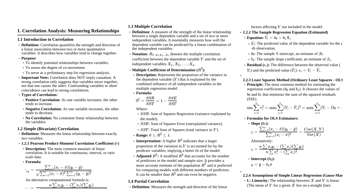
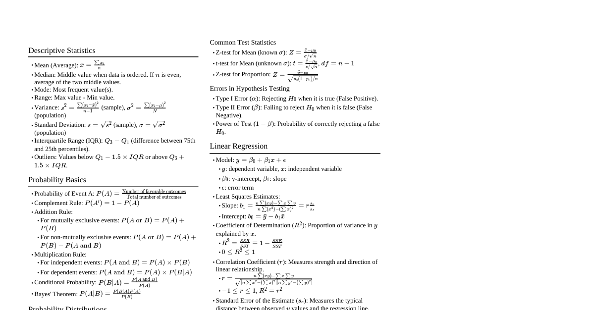
1. Correlation Analysis 1.1 Simple Correlation Measures the strength and direction of a linear relationship between two variables. Pearson's Correlation Coefficient ($r$): This is a measure of the linear correlation between two sets of data. It is the ratio of the covariance of the two variables to the product of their standard deviations. $$r = \frac{n(\sum xy) - (\sum x)(\sum y)}{\sqrt{[n\sum x^2 - (\sum x)^2][n\sum y^2 - (\sum y)^2]}}$$ Range: $-1 \le r \le 1$. $r=1$: Perfect positive linear relationship (as one variable increases, the other increases proportionally). $r=-1$: Perfect negative linear relationship (as one variable increases, the other decreases proportionally). $r=0$: No linear relationship (the variables are not linearly associated, though other non-linear relationships might exist). Interpretation of $r$: $|r| $0.3 \le |r| $|r| \ge 0.7$: Strong linear relationship. Spearman's Rank Correlation Coefficient ($\rho$ or $r_s$): Used for non-parametric data or when the relationship is not necessarily linear but monotonic. It measures the strength and direction of the monotonic relationship between two ranked variables. $$\rho = 1 - \frac{6 \sum d_i^2}{n(n^2 - 1)}$$ $d_i$: Difference between the ranks of corresponding observations. $n$: Number of observations. Coefficient of Determination ($R^2$): $R^2 = r^2$. Represents the proportion of variance in the dependent variable that can be predicted or explained from the independent variable(s). $0 \le R^2 \le 1$. A higher $R^2$ indicates a better fit of the model to the data. 1.2 Multiple Correlation Measures the linear relationship between a dependent variable ($Y$) and a set of two or more independent variables ($X_1, X_2, ..., X_k$). Multiple Correlation Coefficient ($R_{y.x_1x_2...x_k}$): Always non-negative, $0 \le R \le 1$. It quantifies how well the dependent variable can be predicted from the entire set of independent variables. $R^2$ in multiple regression, often called the coefficient of multiple determination, indicates the proportion of total variance in the dependent variable explained by the set of independent variables in the model. Adjusted $R^2$: A modified version of $R^2$ that adjusts for the number of predictors in the model. It increases only if the new term improves the model more than would be expected by chance, making it useful for comparing models with different numbers of predictors. $$R_{adj}^2 = 1 - \left( \frac{(1 - R^2)(n - 1)}{n - k - 1} \right)$$ $n$: Number of observations. $k$: Number of independent variables. 1.3 Partial Correlation Measures the linear relationship between two variables while statistically controlling for the effect of one or more other variables. This helps to isolate the direct relationship between the two variables of interest. Partial Correlation Coefficient ($r_{xy.z}$): The correlation between $X$ and $Y$ with the linear effect of $Z$ removed from both $X$ and $Y$. $$r_{xy.z} = \frac{r_{xy} - r_{xz}r_{yz}}{\sqrt{(1-r_{xz}^2)(1-r_{yz}^2)}}$$ $r_{xy}$: Simple correlation between X and Y. $r_{xz}$: Simple correlation between X and Z. $r_{yz}$: Simple correlation between Y and Z. Interpretation: If $r_{xy.z}$ is significantly different from $r_{xy}$, it implies that $Z$ has a confounding effect on the relationship between $X$ and $Y$. 2. Regression Analysis 2.1 Simple Linear Regression Models the linear relationship between a dependent variable ($Y$) and a single independent variable ($X$). Aims to predict the value of $Y$ based on the value of $X$. Population Regression Model: $Y_i = \beta_0 + \beta_1 X_i + \epsilon_i$ $Y_i$: The dependent variable for the $i^{th}$ observation. $X_i$: The independent variable for the $i^{th}$ observation. $\beta_0$: Y-intercept (the expected value of $Y$ when $X=0$). $\beta_1$: Slope coefficient (the expected change in $Y$ for a one-unit increase in $X$). $\epsilon_i$: Error term (represents the difference between the actual $Y_i$ and the value predicted by the linear model; accounts for unmeasured factors and random variability). Estimated Regression Equation (Sample): $\hat{Y}_i = b_0 + b_1 X_i$ $\hat{Y}_i$: The predicted value of the dependent variable for the $i^{th}$ observation. $b_0$: Sample estimate of $\beta_0$. $b_1$: Sample estimate of $\beta_1$. Least Squares Method: The coefficients $b_0$ and $b_1$ are estimated by minimizing the sum of squared residuals ($\sum (Y_i - \hat{Y}_i)^2$). $b_1 = \frac{n\sum xy - (\sum x)(\sum y)}{n\sum x^2 - (\sum x)^2} = \frac{Cov(X,Y)}{Var(X)}$ $b_0 = \bar{y} - b_1 \bar{x}$ Assumptions of Simple Linear Regression (LINE): L inearity: The relationship between $X$ and $Y$ is linear. I ndependence of errors: The error terms $\epsilon_i$ are independent of each other. N ormality of errors: The error terms $\epsilon_i$ are normally distributed for any given value of $X$. E qual variance of errors (Homoscedasticity): The variance of the error terms is constant across all levels of $X$. Analysis of Variance (ANOVA) for Regression: Total Sum of Squares (SST): $\sum (Y_i - \bar{Y})^2$. Measures total variation in $Y$. Regression Sum of Squares (SSR): $\sum (\hat{Y}_i - \bar{Y})^2$. Measures variation in $Y$ explained by the model. Error Sum of Squares (SSE): $\sum (Y_i - \hat{Y}_i)^2$. Measures variation in $Y$ unexplained by the model. Relationship: $SST = SSR + SSE$. $R^2 = \frac{SSR}{SST}$. 2.2 Introduction to Multiple Regression Models the linear relationship between a dependent variable ($Y$) and two or more independent variables ($X_1, X_2, ..., X_k$). Allows for more complex and realistic modeling of real-world phenomena. Population Multiple Regression Model: $Y_i = \beta_0 + \beta_1 X_{1i} + \beta_2 X_{2i} + ... + \beta_k X_{ki} + \epsilon_i$ $\beta_0$: Y-intercept (expected value of $Y$ when all $X$ variables are zero). $\beta_j$: Partial regression coefficient for $X_j$. It represents the expected change in $Y$ for a one-unit increase in $X_j$, holding all other independent variables constant. Estimated Multiple Regression Equation: $\hat{Y}_i = b_0 + b_1 X_{1i} + b_2 X_{2i} + ... + b_k X_{ki}$ Assumptions: Similar to simple linear regression, but also includes: No perfect multicollinearity: No exact linear relationship among the independent variables. Interpretation of Coefficients: In multiple regression, each $b_j$ is a "partial" coefficient, meaning it reflects the unique effect of $X_j$ on $Y$ after accounting for the effects of all other predictor variables in the model. 3. Theory of Attributes Deals with qualitative characteristics or attributes that cannot be measured numerically but can only be classified (e.g., gender, literacy, smoking habit). Attributes are either present or absent. 3.1 Association of Attributes Examines whether there is a relationship or dependence between two or more attributes. Notation: $N$: Total number of observations. $(A)$, $(B)$: Frequencies of the presence of attributes A and B, respectively. $(\alpha)$, $(\beta)$: Frequencies of the absence of attributes A and B, respectively. $(\alpha) = N - (A)$ $(\beta) = N - (B)$ $(AB)$: Frequency of presence of both A and B. $(A\beta)$: Frequency of presence of A and absence of B. $(\alpha B)$: Frequency of absence of A and presence of B. $(\alpha\beta)$: Frequency of absence of both A and B. Independence of Attributes: Two attributes A and B are independent if the presence or absence of one does not affect the presence or absence of the other. Conditions for independence: $(AB) = \frac{(A)(B)}{N}$ $(A\beta) = \frac{(A)(\beta)}{N}$ $(\alpha B) = \frac{(\alpha)(B)}{N}$ $(\alpha\beta) = \frac{(\alpha)(\beta)}{N}$ Coefficient of Association ($Q$ - Yule's Coefficient): Measures the degree of association between two attributes. $$Q = \frac{(AB)(\alpha\beta) - (A\beta)(\alpha B)}{(AB)(\alpha\beta) + (A\beta)(\alpha B)}$$ Range: $-1 \le Q \le 1$. $Q=1$: Perfect positive association (A and B always occur together). $Q=-1$: Perfect negative association (A and B never occur together). $Q=0$: No association (attributes are independent). Coefficient of Colligation ($K$): Another measure of association, often considered more robust for certain cases. $$K = \frac{\sqrt{(AB)(\alpha\beta)} - \sqrt{(A\beta)(\alpha B)}}{\sqrt{(AB)(\alpha\beta)} + \sqrt{(A\beta)(\alpha B)}}$$ Range: $-1 \le K \le 1$. $K = \frac{2Q}{1+Q^2}$. 3.2 Consistency of Data A set of observed frequencies (class frequencies) derived from attributes is considered consistent if none of the ultimate class frequencies are negative. An ultimate class frequency refers to the frequency of a specific combination of presence/absence for all attributes (e.g., $(AB)$ or $(\alpha\beta)$). For two attributes A and B, the conditions for consistency are: All ultimate class frequencies must be non-negative: $(AB) \ge 0$ $(A\beta) \ge 0 \implies (A) - (AB) \ge 0$ $(\alpha B) \ge 0 \implies (B) - (AB) \ge 0$ $(\alpha\beta) \ge 0 \implies N - (A) - (B) + (AB) \ge 0$ If any of these conditions are violated, the given data set is inconsistent, implying an error in data collection or reporting. 4. Probability Theory 4.1 Basic Concepts Experiment: Any process that produces an observation or outcome. Outcome: A single result of an experiment. Sample Space ($S$ or $\Omega$): The set of all possible outcomes of a random experiment. Event ($E$): A subset of the sample space; a collection of outcomes. Simple Event: An event consisting of a single outcome. Compound Event: An event consisting of more than one outcome. Probability of an Event ($P(E)$): A numerical measure of the likelihood that an event will occur. Classical Definition: $P(E) = \frac{\text{Number of favorable outcomes}}{\text{Total number of possible outcomes}}$ (assuming equally likely outcomes). Relative Frequency Definition: $P(E) = \frac{\text{Number of times E occurs}}{\text{Total number of trials}}$ (as number of trials approaches infinity). Subjective Definition: Based on personal judgment. Axioms of Probability: $0 \le P(E) \le 1$ for any event $E$. $P(S) = 1$ (The probability of the sample space occurring is 1). If $E_1, E_2, ...$ are mutually exclusive events, then $P(E_1 \cup E_2 \cup ...) = P(E_1) + P(E_2) + ...$. Complement of an Event ($E^c$ or $\bar{E}$): The event that $E$ does not occur. $P(E^c) = 1 - P(E)$. Mutually Exclusive Events: Events that cannot occur at the same time ($A \cap B = \emptyset$). Independent Events: Events where the occurrence of one does not affect the probability of the other. 4.2 Addition Theorem (for Union of Events) For any two events A and B (not necessarily mutually exclusive): $$P(A \cup B) = P(A) + P(B) - P(A \cap B)$$ $P(A \cup B)$: Probability that A occurs OR B occurs OR both occur. $P(A \cap B)$: Probability that A and B both occur (intersection). If A and B are mutually exclusive events: $$P(A \cup B) = P(A) + P(B)$$ For three events A, B, C: $$P(A \cup B \cup C) = P(A) + P(B) + P(C) - P(A \cap B) - P(A \cap C) - P(B \cap C) + P(A \cap B \cap C)$$ 4.3 Multiplication Theorem (for Intersection of Events) For any two events A and B: $$P(A \cap B) = P(A) P(B|A)$$ or $$P(A \cap B) = P(B) P(A|B)$$ This is used to find the probability that both A and B occur. If A and B are independent events: $$P(A \cap B) = P(A) P(B)$$ The occurrence of one event does not change the probability of the other. 4.4 Conditional Probability The probability of an event A occurring given that another event B has already occurred ($P(A|B)$). It effectively reduces the sample space to event B. Formula: $$P(A|B) = \frac{P(A \cap B)}{P(B)}, \quad \text{provided } P(B) > 0$$ Similarly, $$P(B|A) = \frac{P(A \cap B)}{P(A)}, \quad \text{provided } P(A) > 0$$ If A and B are independent, then $P(A|B) = P(A)$ and $P(B|A) = P(B)$. 4.5 Bayes' Theorem A fundamental theorem in probability that describes how to update the probability of a hypothesis ($A_i$) based on new evidence ($B$). It relates the conditional probability $P(A|B)$ to $P(B|A)$. Let $A_1, A_2, ..., A_n$ be a set of mutually exclusive and exhaustive events (a partition of the sample space), and $B$ be any other event with $P(B) > 0$. $$P(A_i|B) = \frac{P(B|A_i)P(A_i)}{\sum_{j=1}^{n} P(B|A_j)P(A_j)}$$ $P(A_i)$: Prior probability of event $A_i$. $P(B|A_i)$: Likelihood of observing event $B$ given $A_i$ is true. $P(A_i|B)$: Posterior probability of event $A_i$ given that $B$ has occurred. The denominator is $P(B)$, the total probability of event $B$. 5. Random Variables A random variable is a variable whose value is a numerical outcome of a random phenomenon. Discrete Random Variable: A random variable that can take on a finite or countably infinite number of values (e.g., number of heads in 3 coin flips). Its probability distribution is described by a Probability Mass Function (PMF). Continuous Random Variable: A random variable that can take on any value within a given range (e.g., height, temperature). Its probability distribution is described by a Probability Density Function (PDF). 5.1 Mathematical Expectation (Expected Value) The expected value of a random variable is the weighted average of all possible values it can take, with the weights being their respective probabilities. It represents the "long-run average" or center of the distribution. For a discrete random variable $X$ with PMF $P(X=x_i)$: $$E(X) = \sum_{\text{all } x_i} x_i P(X=x_i)$$ For a continuous random variable $X$ with PDF $f(x)$: $$E(X) = \int_{-\infty}^{\infty} x f(x) dx$$ Expected Value of a Function of a Random Variable $g(X)$: Discrete: $E(g(X)) = \sum_{\text{all } x_i} g(x_i) P(X=x_i)$ Continuous: $E(g(X)) = \int_{-\infty}^{\infty} g(x) f(x) dx$ Properties of Expectation: $E(c) = c$ (for a constant $c$). $E(cX) = c E(X)$ (for a constant $c$). $E(X+Y) = E(X) + E(Y)$ (always true, even if $X$ and $Y$ are not independent). $E(aX+bY) = aE(X) + bE(Y)$ (for constants $a, b$). If $X$ and $Y$ are independent, $E(XY) = E(X)E(Y)$. Variance ($Var(X)$ or $\sigma^2$): Measures the spread or dispersion of a random variable around its mean. $$Var(X) = E[(X - E(X))^2]$$ An easier computational formula: $$Var(X) = E(X^2) - [E(X)]^2$$ Properties of Variance: $Var(c) = 0$ (variance of a constant is zero). $Var(cX) = c^2 Var(X)$. $Var(X+c) = Var(X)$. If $X$ and $Y$ are independent, $Var(X+Y) = Var(X) + Var(Y)$ and $Var(X-Y) = Var(X) + Var(Y)$. $Var(aX+bY) = a^2Var(X) + b^2Var(Y) + 2abCov(X,Y)$. If $X,Y$ are independent, $Cov(X,Y)=0$. Standard Deviation ($\sigma$): $\sigma = \sqrt{Var(X)}$. 6. Theoretical Probability Distributions 6.1 Binomial Distribution Models the number of successes in a fixed number of independent Bernoulli (binary outcome) trials. Conditions for a Binomial Experiment: Fixed number of trials, $n$. Each trial has only two possible outcomes: "success" or "failure". The probability of success, $p$, is constant for each trial. The trials are independent. Parameters: $n$ (number of trials), $p$ (probability of success on a single trial). Probability Mass Function (PMF): For $X$ successes in $n$ trials: $$P(X=k) = \binom{n}{k} p^k (1-p)^{n-k}, \quad \text{for } k=0, 1, ..., n$$ where $\binom{n}{k} = \frac{n!}{k!(n-k)!}$ is the binomial coefficient. Mean (Expected Value): $E(X) = np$ Variance: $Var(X) = np(1-p)$ Standard Deviation: $\sigma_X = \sqrt{np(1-p)}$ 6.2 Poisson Distribution Models the number of events occurring in a fixed interval of time or space, or in a specific area/volume, given that these events occur with a known constant mean rate and independently of the time since the last event. It's often used for rare events. Conditions for a Poisson Experiment: The number of events in an interval is independent of the number of events in any other non-overlapping interval. The probability of an event occurring in a very short interval is proportional to the length of the interval. The probability of more than one event occurring in such a short interval is negligible. Parameter: $\lambda$ (lambda), which is the average rate or mean number of events in the given interval. Probability Mass Function (PMF): For $X$ events: $$P(X=k) = \frac{e^{-\lambda} \lambda^k}{k!}, \quad \text{for } k=0, 1, 2, ...$$ where $e \approx 2.71828$ is Euler's number. Mean (Expected Value): $E(X) = \lambda$ Variance: $Var(X) = \lambda$ Relationship with Binomial: Poisson distribution can approximate binomial distribution when $n$ is large and $p$ is small, with $\lambda = np$. 6.3 Normal Distribution The most widely used continuous probability distribution, often referred to as the "bell curve" or Gaussian distribution. It is symmetric about its mean. Parameters: $\mu$ (mean, which is also the median and mode), $\sigma^2$ (variance). Probability Density Function (PDF): $$f(x) = \frac{1}{\sigma\sqrt{2\pi}} e^{-\frac{1}{2}(\frac{x-\mu}{\sigma})^2}, \quad \text{for } -\infty Properties: Symmetric around its mean $\mu$. The total area under the curve is 1. The curve extends infinitely in both directions, approaching the x-axis but never touching it. The "Empirical Rule" (or 68-95-99.7 Rule): Approximately 68% of the data falls within $1\sigma$ of the mean ($\mu \pm 1\sigma$). Approximately 95% of the data falls within $2\sigma$ of the mean ($\mu \pm 2\sigma$). Approximately 99.7% of the data falls within $3\sigma$ of the mean ($\mu \pm 3\sigma$). Standard Normal Distribution (Z-distribution): A special case of the normal distribution with mean $\mu=0$ and standard deviation $\sigma=1$. Any normal random variable $X$ can be transformed into a standard normal random variable $Z$ using the formula: $$Z = \frac{X-\mu}{\sigma}$$ This transformation allows us to use standard normal tables to find probabilities. 6.4 Goodness of Fit (Chi-square Test) A statistical hypothesis test used to determine how well observed data fits an expected distribution. It tests whether there is a significant difference between the observed frequencies and the frequencies expected under a specific theoretical distribution (e.g., uniform, binomial, Poisson, or even normal, after grouping). Hypotheses: $H_0$: The observed data comes from the specified theoretical distribution (i.e., there is no significant difference between observed and expected frequencies). $H_1$: The observed data does not come from the specified theoretical distribution (i.e., there is a significant difference). Test Statistic ($\chi^2$): $$\chi^2 = \sum_{i=1}^{k} \frac{(O_i - E_i)^2}{E_i}$$ $O_i$: Observed frequency in category $i$. $E_i$: Expected frequency in category $i$ under $H_0$. $k$: Number of categories or classes. Rule of thumb: Each expected frequency $E_i$ should be at least 5. If not, combine categories. Degrees of Freedom ($df$): $df = k - 1 - m$, where $m$ is the number of parameters of the theoretical distribution estimated from the sample data. If no parameters are estimated from the sample (e.g., testing against a known uniform distribution), $m=0$. If one parameter (e.g., $\lambda$ for Poisson or $p$ for Binomial) is estimated, $m=1$. If two parameters (e.g., $\mu$ and $\sigma$ for Normal) are estimated, $m=2$. Decision Rule: Compare the calculated $\chi^2$ value to a critical value from the chi-square distribution table with $df$ degrees of freedom and a chosen significance level $\alpha$. If $\chi^2_{\text{calculated}} > \chi^2_{\text{critical}}$, reject $H_0$. Alternatively, if P-value $\le \alpha$, reject $H_0$. 7. Sampling Theory The study of how to select a representative sample from a population and how to make inferences about the population based on that sample. 7.1 Population and Sample Population (Universe): The entire group of individuals, objects, or data points about which information is desired. It is the complete set of all possible observations. Can be finite (e.g., all students in a university) or infinite (e.g., all possible outcomes of rolling a die). Sample: A subset or a part of the population that is actually selected and observed. It is used to draw conclusions about the entire population. A good sample is representative of the population, meaning its characteristics closely mirror those of the population. 7.2 Parameter and Statistic Parameter: A numerical characteristic or measure that describes a feature of the entire population. Parameters are typically fixed but often unknown. Examples: Population mean ($\mu$), population standard deviation ($\sigma$), population proportion ($p$), population variance ($\sigma^2$). Statistic: A numerical characteristic or measure that describes a feature of a sample. Statistics are calculated from sample data and are used to estimate or make inferences about population parameters. Statistics vary from sample to sample. Examples: Sample mean ($\bar{x}$), sample standard deviation ($s$), sample proportion ($\hat{p}$), sample variance ($s^2$). 7.3 Objectives of Sampling Cost Efficiency: Studying a sample is usually much less expensive than studying the entire population. Time Efficiency: Data collection and analysis from a sample can be completed much faster. Feasibility: For very large or infinite populations, a census is impossible. Sampling provides the only practical way to gather information. Accuracy: In some cases, a carefully conducted sample survey can yield more accurate results than a census, especially when the census is prone to non-sampling errors (e.g., due to the sheer volume of data, poor training of enumerators). Destructive Testing: When the measurement process destroys the item (e.g., testing the lifespan of light bulbs), sampling is essential. 7.4 Types of Sampling Probability Sampling (Random Sampling): Each unit in the population has a known, non-zero probability of being selected, and the selection is based on chance. This allows for statistical inference and estimation of sampling error. Simple Random Sampling (SRS): Every possible sample of a given size $n$ has an equal chance of being selected. Each individual unit has an equal probability of selection. (e.g., drawing names from a hat, using a random number generator). Systematic Sampling: Units are selected from an ordered list at regular intervals. A starting point is chosen randomly, and then every $k^{th}$ unit is selected (e.g., selecting every 10th customer). $k = N/n$. Stratified Sampling: The population is divided into mutually exclusive, homogeneous subgroups called strata (e.g., age groups, gender, income levels). Then, a simple random sample is drawn from each stratum. This ensures representation from all important subgroups. Cluster Sampling: The population is divided into heterogeneous clusters (e.g., geographic areas, schools). A random sample of clusters is selected, and then all units within the selected clusters are included in the sample. Often used for large, geographically dispersed populations. Multistage Sampling: Involves selecting samples in stages (e.g., randomly select states, then randomly select counties within those states, then randomly select households within those counties). Non-Probability Sampling: The selection of units is not based on chance; rather, it relies on the subjective judgment of the researcher. This type of sampling does not allow for generalization to the population or estimation of sampling error. Convenience Sampling: Units are selected based on their ease of accessibility or proximity to the researcher (e.g., surveying people walking by on a street). Quota Sampling: Similar to stratified sampling, but selection within strata is non-random. The researcher sets quotas for different subgroups and then selects units until the quotas are filled (e.g., interview 50 men and 50 women). Purposive (Judgmental) Sampling: The researcher deliberately selects units based on their expert knowledge or specific purpose of the study (e.g., selecting experts in a particular field). Snowball Sampling: Initial participants are asked to identify other potential participants who meet the study criteria. Useful for hard-to-reach populations. 8. Testing of Significance (Hypothesis Testing) A formal procedure for making inferences about population parameters based on sample data. It involves comparing observed sample statistics to what would be expected if a particular hypothesis about the population were true. 8.1 Hypotheses Testing Framework Step 1: State the Hypotheses. Null Hypothesis ($H_0$): A statement of no effect, no difference, or no relationship. It is the statement assumed to be true until there is sufficient evidence to reject it. (e.g., $H_0: \mu = \mu_0$, $H_0: p_1 = p_2$). Alternative Hypothesis ($H_1$ or $H_a$): A statement that contradicts the null hypothesis. It represents what the researcher is trying to find evidence for. (e.g., $H_1: \mu \ne \mu_0$, $H_1: \mu > \mu_0$, $H_1: p_1 Step 2: Choose a Level of Significance ($\alpha$). Step 3: Select the Appropriate Test Statistic. (Depends on the type of data, sample size, population parameters, etc.) Step 4: Determine the Critical Region (or calculate P-value). Step 5: Calculate the Test Statistic from Sample Data. Step 6: Make a Decision. (Compare test statistic to critical value, or P-value to $\alpha$). Step 7: State the Conclusion in Context. 8.2 Type I & Type II Errors When making a decision in hypothesis testing, there are four possible outcomes: $H_0$ is True $H_0$ is False Do Not Reject $H_0$ Correct Decision Type II Error ($\beta$) Reject $H_0$ Type I Error ($\alpha$) Correct Decision (Power) Type I Error ($\alpha$): Rejecting the null hypothesis when it is actually true. This is often called a "false positive." The probability of committing a Type I error is denoted by $\alpha$, which is the chosen level of significance. Controlled by the researcher (e.g., setting $\alpha = 0.05$). Type II Error ($\beta$): Failing to reject the null hypothesis when it is actually false. This is often called a "false negative." The probability of committing a Type II error is denoted by $\beta$. $\beta$ is influenced by sample size, effect size, and $\alpha$. Power of the Test ($1-\beta$): The probability of correctly rejecting a false null hypothesis. It is the probability of detecting an effect if there is an effect to be detected. There is an inverse relationship between $\alpha$ and $\beta$: decreasing one often increases the other. Researchers typically prioritize controlling Type I error. 8.3 Level of Significance ($\alpha$) The maximum acceptable probability of committing a Type I error. It is the threshold for statistical significance. Commonly chosen values are 0.05 (5%), 0.01 (1%), or 0.10 (10%). If the P-value is less than or equal to $\alpha$, we reject $H_0$. 8.4 Confidence Level ($1-\alpha$) The probability that a confidence interval will contain the true population parameter if the sampling and estimation process were repeated many times. It is directly related to the level of significance: Confidence Level = $1 - \alpha$. Common confidence levels: 95%, 99%, 90%. A 95% confidence level means that if we were to take many samples and construct a confidence interval for each, approximately 95% of these intervals would contain the true population parameter. 8.5 Critical Region (Rejection Region) The set of values for the test statistic that leads to the rejection of the null hypothesis. It is determined by the chosen level of significance ($\alpha$) and the sampling distribution of the test statistic. The boundaries of the critical region are called critical values. 8.6 Interpretation of P-Value The P-value (probability value) is the probability of obtaining a test statistic as extreme as, or more extreme than, the one observed from the sample, *assuming that the null hypothesis is true*. It quantifies the strength of evidence against the null hypothesis. A small P-value means the observed data is unlikely under $H_0$, providing strong evidence to reject $H_0$. Decision Rule using P-value: If P-value $\le \alpha$: Reject $H_0$. (The result is statistically significant, meaning the observed difference is unlikely due to chance alone if $H_0$ were true). If P-value $> \alpha$: Fail to reject $H_0$. (The result is not statistically significant, meaning there isn't enough evidence to conclude $H_0$ is false). Note: "Failing to reject $H_0$" is not the same as "accepting $H_0$". It simply means the data does not provide sufficient evidence to conclude $H_0$ is false. 8.7 One-tailed and Two-tailed Tests The type of test depends on the alternative hypothesis. Two-tailed Test: $H_1$ specifies a difference or effect in either direction (e.g., $H_1: \mu \ne \mu_0$). The critical region is split into two parts, one in each tail of the sampling distribution. $\alpha$ is divided by 2 for each tail (e.g., for $\alpha=0.05$, $0.025$ in each tail). One-tailed Test (Left-tailed): $H_1$ specifies a difference in a specific negative direction (e.g., $H_1: \mu The entire critical region is in the left tail of the sampling distribution. One-tailed Test (Right-tailed): $H_1$ specifies a difference in a specific positive direction (e.g., $H_1: \mu > \mu_0$). The entire critical region is in the right tail of the sampling distribution. One-tailed tests are used when there is a strong theoretical or practical reason to hypothesize a direction. Otherwise, two-tailed tests are generally more conservative and preferred. 8.8 Sampling Distribution - Standard Error Sampling Distribution: The probability distribution of a statistic (e.g., sample mean, sample proportion) obtained from all possible samples of a specific size taken from a population. It describes the variability of the statistic from sample to sample. Central Limit Theorem (CLT): A fundamental theorem stating that, for a sufficiently large sample size ($n \ge 30$ is a common rule of thumb), the sampling distribution of the sample mean (and other statistics) will be approximately normally distributed, regardless of the shape of the original population distribution. Mean of the sampling distribution of $\bar{X}$ is $\mu$. Standard deviation of the sampling distribution of $\bar{X}$ is $\sigma/\sqrt{n}$. Standard Error (SE): The standard deviation of a sampling distribution of a statistic. It measures the typical amount of sampling error or the precision of the sample statistic as an estimate of the population parameter. A smaller standard error indicates a more precise estimate. Standard Error of the Mean ($SE_{\bar{x}}$): When population standard deviation $\sigma$ is known: $SE_{\bar{x}} = \frac{\sigma}{\sqrt{n}}$ When $\sigma$ is unknown (and $n$ is large, or for small $n$ using t-distribution): $SE_{\bar{x}} = \frac{s}{\sqrt{n}}$, where $s$ is the sample standard deviation. Standard Error of the Proportion ($SE_{\hat{p}}$): For population proportion $p$: $SE_{\hat{p}} = \sqrt{\frac{p(1-p)}{n}}$ For sample proportion $\hat{p}$ (used in confidence intervals): $SE_{\hat{p}} = \sqrt{\frac{\hat{p}(1-\hat{p})}{n}}$ 9. Estimation The process of using sample data to estimate unknown population parameters. 9.1 Point Estimates A single value (a statistic) calculated from sample data that serves as the "best guess" or single most likely value for an unknown population parameter. Examples of common point estimators and their corresponding parameters: Sample Mean ($\bar{x}$) is a point estimate for Population Mean ($\mu$). Sample Proportion ($\hat{p}$) is a point estimate for Population Proportion ($p$). Sample Standard Deviation ($s$) is a point estimate for Population Standard Deviation ($\sigma$). Sample Variance ($s^2$) is a point estimate for Population Variance ($\sigma^2$). (Note: $s^2 = \frac{\sum (x_i - \bar{x})^2}{n-1}$ is an unbiased estimator for $\sigma^2$). While simple, point estimates do not convey information about the precision or reliability of the estimate. 9.2 Interval Estimates (Confidence Intervals) A range of values within which the true population parameter is expected to lie, with a certain level of confidence. It provides both an estimated value and a measure of its precision. General Form of a Confidence Interval: $$\text{Point Estimate} \pm (\text{Critical Value} \times \text{Standard Error of the Estimate})$$ $$\text{Point Estimate} \pm \text{Margin of Error}$$ Confidence Interval for Population Mean ($\mu$): Large Sample ($n \ge 30$) or $\sigma$ known (using Z-distribution): $$\bar{x} \pm Z_{\alpha/2} \frac{\sigma}{\sqrt{n}}$$ If $\sigma$ is unknown but $n \ge 30$, use $s$ as an estimate for $\sigma$: $$\bar{x} \pm Z_{\alpha/2} \frac{s}{\sqrt{n}}$$ Small Sample ($n $$\bar{x} \pm t_{\alpha/2, df} \frac{s}{\sqrt{n}}$$ where $df = n-1$. Confidence Interval for Population Proportion ($p$) (Large Sample): Requires $np \ge 10$ and $n(1-p) \ge 10$ (or $n\hat{p} \ge 10$ and $n(1-\hat{p}) \ge 10$). $$\hat{p} \pm Z_{\alpha/2} \sqrt{\frac{\hat{p}(1-\hat{p})}{n}}$$ Interpretation: A 95% confidence interval for $\mu$ means that if we were to take many samples and construct a confidence interval from each, approximately 95% of these intervals would contain the true population mean $\mu$. It does NOT mean there is a 95% chance that the true mean falls within *this specific* interval. 9.3 Characteristics of a Good Estimator An estimator $\hat{\theta}$ for a parameter $\theta$ is considered "good" if it possesses several desirable statistical properties: Unbiasedness: An estimator is unbiased if its expected value is equal to the true population parameter it is estimating. $$E(\hat{\theta}) = \theta$$ Example: $E(\bar{x}) = \mu$, so $\bar{x}$ is an unbiased estimator of $\mu$. Example: $E(s^2) = \sigma^2$, so $s^2$ is an unbiased estimator of $\sigma^2$. (Note: $s$ is a biased estimator of $\sigma$, but the bias is often small for large samples). Consistency: An estimator is consistent if, as the sample size ($n$) increases, the estimator converges in probability to the true parameter value. This means that with larger samples, the estimate becomes more accurate and reliable. Efficiency: An unbiased estimator is considered efficient if it has the smallest variance among all possible unbiased estimators for the same parameter. A more efficient estimator provides a more precise estimate (less spread in its sampling distribution). The Cramér-Rao Lower Bound defines the minimum possible variance for an unbiased estimator. Sufficiency: An estimator is sufficient if it utilizes all the information about the population parameter that is contained in the sample. In other words, no other statistic calculated from the same sample can provide additional information about the parameter. 10. Large Sample Tests ($n \ge 30$) For large samples, the Central Limit Theorem allows us to assume that the sampling distributions of many statistics are approximately normal, even if the population distribution is not normal. This allows the use of Z-tests. 10.1 Distribution of Sample Mean (Z-test for Mean) Hypothesis Testing for a Single Population Mean ($\mu$): $H_0: \mu = \mu_0$ $H_1: \mu \ne \mu_0$ (two-tailed), or $\mu > \mu_0$ (right-tailed), or $\mu Test Statistic (if $\sigma$ is known): $$Z = \frac{\bar{x} - \mu_0}{\sigma/\sqrt{n}}$$ Test Statistic (if $\sigma$ is unknown, but $n \ge 30$): We can substitute $s$ for $\sigma$. $$Z = \frac{\bar{x} - \mu_0}{s/\sqrt{n}}$$ Hypothesis Testing for Difference Between Two Population Means ($\mu_1 - \mu_2$): (Independent Samples) $H_0: \mu_1 = \mu_2$ (or $\mu_1 - \mu_2 = 0$) $H_1: \mu_1 \ne \mu_2$, or $\mu_1 > \mu_2$, or $\mu_1 Test Statistic (if $\sigma_1, \sigma_2$ are known): $$Z = \frac{(\bar{x}_1 - \bar{x}_2) - (\mu_1 - \mu_2)}{\sqrt{\frac{\sigma_1^2}{n_1} + \frac{\sigma_2^2}{n_2}}}$$ (Under $H_0$, $\mu_1 - \mu_2 = 0$) Test Statistic (if $\sigma_1, \sigma_2$ are unknown, but $n_1, n_2 \ge 30$): Substitute $s_1, s_2$ for $\sigma_1, \sigma_2$. $$Z = \frac{(\bar{x}_1 - \bar{x}_2)}{\sqrt{\frac{s_1^2}{n_1} + \frac{s_2^2}{n_2}}}$$ 10.2 Distribution of Sample Proportion (Z-test for Proportion) Hypothesis Testing for a Single Population Proportion ($p$): $H_0: p = p_0$ $H_1: p \ne p_0$, or $p > p_0$, or $p Test Statistic: (Requires $np_0 \ge 10$ and $n(1-p_0) \ge 10$) $$Z = \frac{\hat{p} - p_0}{\sqrt{\frac{p_0(1-p_0)}{n}}}$$ where $\hat{p} = x/n$ (number of successes / sample size). Hypothesis Testing for Difference Between Two Population Proportions ($p_1 - p_2$): (Independent Samples) $H_0: p_1 = p_2$ (or $p_1 - p_2 = 0$) $H_1: p_1 \ne p_2$, or $p_1 > p_2$, or $p_1 Test Statistic: (Requires $n_1p_1 \ge 10, n_1(1-p_1) \ge 10, n_2p_2 \ge 10, n_2(1-p_2) \ge 10$) $$Z = \frac{(\hat{p}_1 - \hat{p}_2)}{\sqrt{\hat{p}_{pooled}(1-\hat{p}_{pooled})(\frac{1}{n_1} + \frac{1}{n_2})}}$$ where $\hat{p}_{pooled} = \frac{x_1 + x_2}{n_1 + n_2}$ (pooled sample proportion). 10.3 Chi-square Test ($\chi^2$) Chi-square Test for Independence (Association): Used to determine if there is a statistically significant association between two categorical variables in a contingency table. $H_0$: The two variables are independent (no association). $H_1$: The two variables are dependent (associated). Test Statistic: $$\chi^2 = \sum_{i=1}^{r} \sum_{j=1}^{c} \frac{(O_{ij} - E_{ij})^2}{E_{ij}}$$ $O_{ij}$: Observed frequency in cell $(i,j)$. $E_{ij}$: Expected frequency in cell $(i,j)$ under $H_0$. $$E_{ij} = \frac{(\text{row } i \text{ total}) \times (\text{column } j \text{ total})}{\text{Grand Total}}$$ $r$: Number of rows, $c$: Number of columns. Degrees of Freedom ($df$): $(r-1)(c-1)$. Conditions: All expected frequencies $E_{ij}$ should be at least 5 (or no more than 20% of cells have $E_{ij} Chi-square Test for Goodness of Fit: (See Section 6.4) Chi-square Test for Variance of a Single Population: Used to test hypotheses about the population variance ($\sigma^2$). $H_0: \sigma^2 = \sigma_0^2$ $H_1: \sigma^2 \ne \sigma_0^2$, or $\sigma^2 > \sigma_0^2$, or $\sigma^2 Test Statistic: $$\chi^2 = \frac{(n-1)s^2}{\sigma_0^2}$$ Degrees of Freedom ($df$): $n-1$. Assumption: The population from which the sample is drawn must be normally distributed. 11. Small Sample Tests ($n When the sample size is small and the population standard deviation ($\sigma$) is unknown, the Z-distribution is no longer appropriate. Instead, we use the t-distribution, F-distribution, or Chi-square distribution, which account for the increased uncertainty due to small sample sizes. Key Assumption: For t-tests and F-tests, the population(s) from which the sample(s) are drawn should be approximately normally distributed. 11.1 Testing of Hypothesis of Mean (t-test) The t-distribution is symmetric and bell-shaped like the normal distribution, but it has heavier tails, meaning it accounts for more variability in smaller samples. It is characterized by its degrees of freedom ($df$). Single Sample t-test: Used to test if a sample mean ($\bar{x}$) is significantly different from a hypothesized population mean ($\mu_0$). $H_0: \mu = \mu_0$ $H_1: \mu \ne \mu_0$, or $\mu > \mu_0$, or $\mu Test Statistic: $$t = \frac{\bar{x} - \mu_0}{s/\sqrt{n}}$$ Degrees of Freedom ($df$): $n-1$. Independent Samples t-test (Two-sample t-test): Used to compare the means of two independent groups. $H_0: \mu_1 = \mu_2$ (or $\mu_1 - \mu_2 = 0$) $H_1: \mu_1 \ne \mu_2$, or $\mu_1 > \mu_2$, or $\mu_1 Assumptions: Independent samples, normally distributed populations, and (often) equal population variances. Test Statistic (Equal Variances Assumed - Pooled t-test): $$t = \frac{(\bar{x}_1 - \bar{x}_2) - (\mu_1 - \mu_2)}{\sqrt{s_p^2 (\frac{1}{n_1} + \frac{1}{n_2})}}$$ where $s_p^2 = \frac{(n_1-1)s_1^2 + (n_2-1)s_2^2}{n_1+n_2-2}$ is the pooled variance. (Under $H_0$, $\mu_1 - \mu_2 = 0$). Degrees of Freedom ($df$): $n_1 + n_2 - 2$. Test Statistic (Unequal Variances Not Assumed - Welch's t-test): More complex formula for $df$, often calculated by software. Typically used when variances are significantly different. Paired Samples t-test: Used to compare the means of two related groups or measurements from the same subjects under two different conditions (e.g., before-after treatment). It analyzes the differences between paired observations. $H_0: \mu_d = 0$ (The mean difference is zero) $H_1: \mu_d \ne 0$, or $\mu_d > 0$, or $\mu_d Let $d_i = x_{1i} - x_{2i}$ be the difference for each pair. Calculate $\bar{d}$ (mean of differences) and $s_d$ (standard deviation of differences). Test Statistic: $$t = \frac{\bar{d} - \mu_d}{s_d/\sqrt{n}}$$ (Under $H_0$, $\mu_d = 0$). Degrees of Freedom ($df$): $n-1$, where $n$ is the number of pairs. 11.2 Testing of Hypothesis of Variance (F-test) The F-distribution is used when comparing variances. It is a positively skewed distribution, characterized by two degrees of freedom (numerator and denominator). F-test for Equality of Two Population Variances ($\sigma_1^2, \sigma_2^2$): Used to determine if the variances of two normally distributed populations are equal. This test is often a precursor to choosing between pooled and unpooled t-tests for means. $H_0: \sigma_1^2 = \sigma_2^2$ $H_1: \sigma_1^2 \ne \sigma_2^2$ (two-tailed), or $\sigma_1^2 > \sigma_2^2$ (right-tailed) Test Statistic: $$F = \frac{s_1^2}{s_2^2}$$ Conventionally, the larger sample variance is placed in the numerator to ensure $F \ge 1$. Degrees of Freedom: $df_1 = n_1-1$ (for the numerator variance), $df_2 = n_2-1$ (for the denominator variance). Assumption: Both populations must be normally distributed. 11.3 Testing of Hypothesis of Correlation Coefficient (t-test) Used to test whether the population correlation coefficient ($\rho$) between two variables is significantly different from zero, implying a linear relationship. Hypotheses: $H_0: \rho = 0$ (No linear relationship in the population) $H_1: \rho \ne 0$, or $\rho > 0$, or $\rho Test Statistic: $$t = \frac{r\sqrt{n-2}}{\sqrt{1-r^2}}$$ where $r$ is the sample Pearson correlation coefficient. Degrees of Freedom ($df$): $n-2$. Assumption: The data come from a bivariate normal distribution. 11.4 Testing of Hypothesis of Regression Coefficient (t-test for Slope) In simple linear regression, this test determines if the independent variable ($X$) has a statistically significant linear effect on the dependent variable ($Y$) in the population. It tests if the population slope ($\beta_1$) is different from zero. Hypotheses: $H_0: \beta_1 = 0$ (No linear relationship between $X$ and $Y$) $H_1: \beta_1 \ne 0$, or $\beta_1 > 0$, or $\beta_1 Test Statistic: $$t = \frac{b_1 - \beta_{1,0}}{SE_{b_1}}$$ (Under $H_0$, $\beta_{1,0} = 0$, so $t = \frac{b_1}{SE_{b_1}}$) $b_1$: Sample regression slope coefficient. $\beta_{1,0}$: Hypothesized population slope (usually 0). $SE_{b_1}$: Standard error of the sample slope coefficient. $$SE_{b_1} = \frac{s_{e}}{\sqrt{\sum(x_i - \bar{x})^2}}$$ where $s_e = \sqrt{\frac{SSE}{n-2}} = \sqrt{\frac{\sum(y_i - \hat{y}_i)^2}{n-2}}$ is the standard error of the estimate (or residual standard error). Degrees of Freedom ($df$): $n-2$. Assumptions: Same as for simple linear regression (LINE assumptions).