Statistics Cheatsheet

Cheatsheet Content

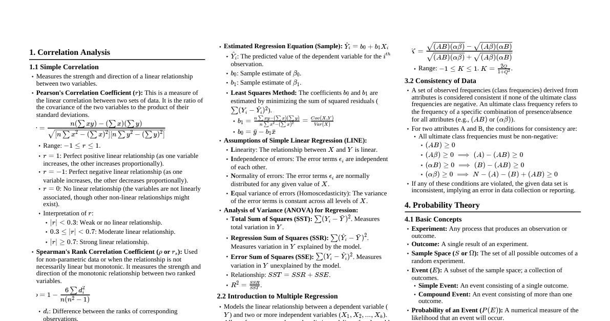
1. Correlation Analysis: Measuring Relationships 1.1 Introduction to Correlation Definition: Correlation quantifies the strength and direction of a linear association between two or more quantitative variables. It describes how variables tend to change together. Purpose: To identify potential relationships between variables. To assess the degree of co-movement. To serve as a preliminary step for regression analysis. Important Note: Correlation does NOT imply causation. A strong correlation only suggests that variables move together, not that one causes the other. Confounding variables or sheer coincidence can lead to strong correlations. Types of Correlation: Positive Correlation: As one variable increases, the other tends to increase. Negative Correlation: As one variable increases, the other tends to decrease. No Correlation: No consistent linear relationship between the variables. 1.2 Simple (Bivariate) Correlation Definition: Measures the linear relationship between exactly two variables. 1.2.1 Pearson Product-Moment Correlation Coefficient ($r$) Description: The most common measure of linear correlation. It is suitable for continuous, interval, or ratio scale data. Formula: $$r_{xy} = \frac{\sum_{i=1}^n (x_i - \bar{x})(y_i - \bar{y})}{\sqrt{\sum_{i=1}^n (x_i - \bar{x})^2 \sum_{i=1}^n (y_i - \bar{y})^2}}$$ An alternative computational formula is: $$r_{xy} = \frac{n \sum x_i y_i - (\sum x_i)(\sum y_i)}{\sqrt{[n \sum x_i^2 - (\sum x_i)^2][n \sum y_i^2 - (\sum y_i)^2]}}$$ Where: $n$: Number of paired observations. $x_i, y_i$: Individual data points. $\bar{x}, \bar{y}$: Sample means of $X$ and $Y$. Range: $-1 \le r \le +1$. $r = +1$: Perfect positive linear correlation. $r = -1$: Perfect negative linear correlation. $r = 0$: No linear correlation. Interpretation of Magnitude: $|r| \in [0, 0.2)$: Very weak or negligible linear relationship. $|r| \in [0.2, 0.4)$: Weak linear relationship. $|r| \in [0.4, 0.6)$: Moderate linear relationship. $|r| \in [0.6, 0.8)$: Strong linear relationship. $|r| \in [0.8, 1.0]$: Very strong linear relationship. Assumptions for Inference (Hypothesis Testing): Quantitative Data: Both variables are measured on an interval or ratio scale. Linearity: The relationship between variables is linear. Independence: Observations are independent. Bivariate Normality: The two variables follow a bivariate normal distribution (for hypothesis testing and confidence intervals). This implies that each variable is normally distributed and that the relationship between them is linear. Homoscedasticity: The variability of data points around the regression line is constant. Coefficient of Determination ($R^2$): For simple linear regression, $R^2 = r^2$. It represents the proportion of variance in one variable that can be explained by the other variable. 1.2.2 Spearman's Rank Correlation Coefficient ($\rho$ or $r_s$) Description: A non-parametric measure of the strength and direction of the monotonic relationship between two ranked variables. It is used for ordinal data or when the assumptions for Pearson correlation (especially normality or linearity) are violated. Formula: $$\rho = 1 - \frac{6 \sum d_i^2}{n(n^2 - 1)}$$ Where: $d_i$: The difference between the ranks of the $i$-th observation for the two variables. $n$: Number of observations. Steps: Rank the data for each variable separately. Calculate the difference ($d_i$) between the ranks for each pair of observations. Square each difference ($d_i^2$). Sum the squared differences. Apply the formula. Range & Interpretation: Same as Pearson's $r$ (from -1 to +1), but interpreted for monotonic (not necessarily linear) relationships between ranks. Assumptions: Data are at least ordinal. Observations are independent. The relationship is monotonic (consistently increasing or decreasing, but not necessarily linear). 1.3 Multiple Correlation Definition: A measure of the strength of the linear relationship between a single dependent variable and a set of two or more independent variables. It essentially measures how well the dependent variable can be predicted by a linear combination of the independent variables. Notation: $R_{Y.X_1X_2...X_k}$ denotes the multiple correlation coefficient between the dependent variable $Y$ and the set of independent variables $X_1, X_2, \dots, X_k$. Multiple Coefficient of Determination ($R^2$): Description: Represents the proportion of the variance in the dependent variable ($Y$) that is explained by the combined influence of all independent variables in the multiple regression model. Formula: $$R^2 = \frac{SSR}{SST} = 1 - \frac{SSE}{SST}$$ Where: $SSR$: Sum of Squares Regression (variance explained by the model). $SSE$: Sum of Squares Error (unexplained variance). $SST$: Total Sum of Squares (total variance in $Y$). Range: $0 \le R^2 \le 1$. Interpretation: A higher $R^2$ indicates that a larger proportion of the variation in $Y$ is accounted for by the predictor variables, implying a better fit of the model. Adjusted $R^2$: A modified $R^2$ that accounts for the number of predictors in the model and sample size. It provides a more accurate estimate of the population $R^2$ and is preferred for comparing models with different numbers of predictors. It can be smaller than $R^2$ and can even be negative. 1.4 Partial Correlation Definition: Measures the strength and direction of the linear relationship between two variables after statistically controlling for (removing the influence of) one or more other variables. It helps to isolate the unique relationship between two variables. Notation: $r_{XY.Z}$ denotes the partial correlation between $X$ and $Y$, controlling for $Z$. $r_{XY.Z_1Z_2}$ controls for $Z_1$ and $Z_2$. Formula (for one control variable $Z$): $$r_{xy.z} = \frac{r_{xy} - r_{xz} r_{yz}}{\sqrt{(1 - r_{xz}^2)(1 - r_{yz}^2)}}$$ Where: $r_{xy}$: Simple correlation between $X$ and $Y$. $r_{xz}$: Simple correlation between $X$ and $Z$. $r_{yz}$: Simple correlation between $Y$ and $Z$. Purpose: To eliminate spurious correlations (where a third variable is driving the relationship). To identify direct relationships between variables by removing the effect of confounding factors. Range & Interpretation: Same as Pearson's $r$ (from -1 to +1). Assumptions: Assumes a linear relationship between all pairs of variables and bivariate normality for inference. 2. Regression Analysis: Modeling Relationships 2.1 Introduction to Regression Analysis Definition: A statistical methodology for estimating the relationships among variables. It focuses on modeling the relationship between a dependent variable and one or more independent variables. Purpose: Prediction/Forecasting: To predict the value of the dependent variable based on the values of the independent variable(s). Explanation: To understand how the dependent variable changes when any one of the independent variables is varied, while the other independent variables are held fixed. Hypothesis Testing: To test hypotheses about the relationships between variables. Key Terms: Dependent Variable (Response Variable, $Y$): The variable whose variation is being explained or predicted. Independent Variable (Predictor Variable, Explanatory Variable, $X$): The variable(s) used to explain or predict the dependent variable. Regression Coefficients ($\beta$): Parameters that quantify the impact of independent variables on the dependent variable. 2.2 Simple Linear Regression (SLR) Definition: A statistical method that models the linear relationship between a single dependent variable ($Y$) and a single independent variable ($X$). 2.2.1 The Population Regression Model Equation: $Y_i = \beta_0 + \beta_1 X_i + \epsilon_i$ $Y_i$: The value of the dependent variable for the $i$-th observation. $\beta_0$: The population Y-intercept, representing the expected value of $Y$ when $X=0$. $\beta_1$: The population slope coefficient, representing the expected change in $Y$ for a one-unit increase in $X$. $X_i$: The value of the independent variable for the $i$-th observation. $\epsilon_i$: The random error term (or residual), representing the unexplained variation in $Y$. It accounts for all other factors affecting $Y$ not included in the model. 2.2.2 The Sample Regression Equation (Estimated) Equation: $\hat{Y}_i = b_0 + b_1 X_i$ $\hat{Y}_i$: The predicted value of the dependent variable for the $i$-th observation. $b_0$: The sample Y-intercept, an estimate of $\beta_0$. $b_1$: The sample slope coefficient, an estimate of $\beta_1$. Residual ($e_i$): The difference between the observed value ($Y_i$) and the predicted value ($\hat{Y}_i$): $e_i = Y_i - \hat{Y}_i$. 2.2.3 Least Squares Method (Ordinary Least Squares - OLS) Principle: The most common method for estimating the regression coefficients ($b_0$ and $b_1$). It chooses the values of $b_0$ and $b_1$ that minimize the sum of the squared residuals (SSE). $$\min \sum_{i=1}^n e_i^2 = \min \sum_{i=1}^n (Y_i - \hat{Y}_i)^2 = \min \sum_{i=1}^n (Y_i - (b_0 + b_1 X_i))^2$$ Formulas for OLS Estimators: Slope ($b_1$): $$b_1 = \frac{\sum_{i=1}^n (x_i - \bar{x})(y_i - \bar{y})}{\sum_{i=1}^n (x_i - \bar{x})^2} = \frac{Cov(X,Y)}{Var(X)}$$ Alternatively: $$b_1 = \frac{n \sum x_i y_i - (\sum x_i)(\sum y_i)}{n \sum x_i^2 - (\sum x_i)^2}$$ Intercept ($b_0$): $$b_0 = \bar{y} - b_1 \bar{x}$$ 2.2.4 Assumptions of Simple Linear Regression (Gauss-Markov Assumptions) L: Linearity: The relationship between $X$ and $Y$ is linear. (The mean of $Y$ for a given $X$ lies on a straight line). I: Independence of Errors: The error terms $\epsilon_i$ are independent of each other. (No correlation between residuals). N: Normality of Errors: The error terms $\epsilon_i$ are normally distributed for any given value of $X$. This is crucial for hypothesis testing and confidence intervals of coefficients. E: Equal Variance of Errors (Homoscedasticity): The variance of the error terms ($\sigma^2$) is constant for all values of $X$. (The spread of residuals is consistent across the range of $X$). No Measurement Error: The independent variable $X$ is measured without error. 2.2.5 Coefficient of Determination ($R^2$) Definition: In SLR, $R^2 = r^2$. It quantifies the proportion of the total variation in the dependent variable ($Y$) that is explained by the independent variable ($X$). Formula: $R^2 = \frac{SSR}{SST} = 1 - \frac{SSE}{SST}$ Interpretation: An $R^2$ of 0.70 means that 70% of the variation in $Y$ can be explained by the linear relationship with $X$. 2.3 Introduction to Multiple Linear Regression (MLR) Definition: An extension of SLR that models the linear relationship between a single dependent variable ($Y$) and two or more independent variables ($X_1, X_2, \dots, X_k$). 2.3.1 The Population Regression Model Equation: $Y_i = \beta_0 + \beta_1 X_{1i} + \beta_2 X_{2i} + \dots + \beta_k X_{ki} + \epsilon_i$ $\beta_j$: The population partial slope coefficient for $X_j$, representing the expected change in $Y$ for a one-unit increase in $X_j$, holding all other independent variables constant. 2.3.2 The Sample Regression Equation (Estimated) Equation: $\hat{Y}_i = b_0 + b_1 X_{1i} + b_2 X_{2i} + \dots + b_k X_{ki}$ Interpretation of Coefficients ($b_j$): Each $b_j$ is the estimated change in $Y$ for a one-unit increase in $X_j$, assuming all other $X$ variables are held constant (ceteris paribus). This is why they are called "partial" regression coefficients. 2.3.3 Estimation: OLS methods are extended to MLR, involving matrix algebra to solve for the $b_j$ coefficients. 2.3.4 Assumptions of Multiple Linear Regression: Linearity: The relationship between $Y$ and each $X_j$ is linear. Independence of Errors: Errors are independent. Normality of Errors: Errors are normally distributed. Homoscedasticity: Constant variance of errors. No Multicollinearity: Independent variables are not highly correlated with each other. High multicollinearity can lead to unstable and unreliable coefficient estimates, making it difficult to interpret the individual impact of each predictor. No Measurement Error: Independent variables are measured without error. 2.3.5 Coefficient of Multiple Determination ($R^2$) and Adjusted $R^2$: As discussed in Section 1.3, $R^2$ indicates the proportion of variance in $Y$ explained by all $X$ variables. Adjusted $R^2$: Crucial in MLR. It penalizes the inclusion of unnecessary predictors, as $R^2$ always increases or stays the same with the addition of more variables, even if they are not truly helpful. Adjusted $R^2$ can decrease if a new variable does not improve the model sufficiently. 2.3.6 Model Selection: Techniques like stepwise regression (forward, backward, bidirectional), best subsets regression, and information criteria (AIC, BIC) are used to select the optimal set of predictors. 3. Theory of Attributes: Qualitative Data Analysis 3.1 Introduction to Attributes Definition: Attributes are qualitative characteristics that cannot be measured numerically but can only be classified into categories or described by their presence or absence. (e.g., gender, marital status, literacy, disease status, pass/fail). Contrast with Variables: Variables are quantitative and measurable (e.g., height, weight, income). Purpose: To analyze relationships and patterns within categorical data. Features: Dichotomous Attributes: Can take only two values (e.g., Male/Female, Yes/No, Present/Absent). Polytomous Attributes: Can take more than two values (e.g., Blood Group A/B/AB/O, Socio-economic status: Low/Medium/High). For analysis, polytomous attributes are often broken down into dichotomous ones. Notation: Attributes are denoted by capital letters (A, B, C, ...). The absence of an attribute is denoted by Greek letters ($\alpha, \beta, \gamma, ...$). Frequencies: The number of observations possessing certain attributes are called class frequencies. $(A)$ denotes the number of units possessing attribute A. $(AB)$ denotes the number of units possessing both A and B. 3.2 Association of Attributes Definition: Investigates whether there is a relationship or dependence between two or more attributes. If the attributes are not independent, they are said to be associated. 3.2.1 Contingency Tables Description: Attributes data are typically presented in contingency tables, which show the frequencies of observations for different combinations of attribute categories. Example: $2 \times 2$ Contingency Table for two attributes A and B: B $\beta$ (not B) Total A $(AB)$ $(A\beta)$ $(A)$ $\alpha$ (not A) $(\alpha B)$ $(\alpha \beta)$ $(\alpha)$ Total $(B)$ $(\beta)$ $N$ Where: $(AB)$: Number of units possessing both A and B. $(A\beta)$: Number of units possessing A but not B. $(\alpha B)$: Number of units possessing B but not A. $(\alpha \beta)$: Number of units possessing neither A nor B. $(A) = (AB) + (A\beta)$: Total number of units possessing A. $(B) = (AB) + (\alpha B)$: Total number of units possessing B. $N = (A) + (\alpha) = (B) + (\beta) = (AB) + (A\beta) + (\alpha B) + (\alpha \beta)$: Total number of observations. 3.2.2 Measures of Association Yule's Coefficient of Association ($Q$): Description: A measure of association for $2 \times 2$ contingency tables. It is based on the ratio of cross-products of cell frequencies. Formula: $$Q = \frac{(AB)(\alpha\beta) - (A\beta)(\alpha B)}{(AB)(\alpha\beta) + (A\beta)(\alpha B)}$$ Range: $-1 \le Q \le +1$. $Q = +1$: Perfect positive association (A and B always occur together). $Q = -1$: Perfect negative association (A and B never occur together). $Q = 0$: No association (attributes are independent). Features: Useful for binary attributes. It's not affected by the sample size or the marginal totals, making it relatively robust. However, it can give a strong association even if frequencies in some cells are very small. Coefficient of Colligation ($K$): Description: Another measure of association, often considered more stable than $Q$ when some cell frequencies are zero. Formula: $$K = \frac{\sqrt{(AB)(\alpha\beta)} - \sqrt{(A\beta)(\alpha B)}}{\sqrt{(AB)(\alpha\beta)} + \sqrt{(A\beta)(\alpha B)}}$$ Relationship to Q: $Q = \frac{2K}{1+K^2}$ Range: $-1 \le K \le +1$. Interpretation is similar to $Q$. Chi-square Test for Independence: While not a measure of association, the Chi-square test (discussed in Section 9.1.3) is used to statistically determine if an association exists between two categorical variables. 3.3 Consistency of Data Definition: A set of observed frequencies (class frequencies) is said to be consistent if they do not violate any fundamental laws of probability or logic, meaning that no theoretical frequency should be negative. Conditions for Consistency (for two attributes A and B): All class frequencies of order zero and one must be non-negative: $(A) \ge 0$, $(B) \ge 0$, $(\alpha) \ge 0$, $(\beta) \ge 0$ All class frequencies of higher orders must be non-negative: $(AB) \ge 0$, $(A\beta) \ge 0$, $(\alpha B) \ge 0$, $(\alpha \beta) \ge 0$ In addition, the following fundamental inequalities must hold: $(AB) \le (A)$ and $(AB) \le (B)$ $(\alpha B) \le (\alpha)$ and $(\alpha B) \le (B)$ $(A\beta) \le (A)$ and $(A\beta) \le (\beta)$ $(\alpha \beta) \le (\alpha)$ and $(\alpha \beta) \le (\beta)$ General conditions derived from the above for a $2 \times 2$ table: $(AB) \ge 0$ $(A) - (AB) \ge 0 \implies (A\beta) \ge 0$ $(B) - (AB) \ge 0 \implies (\alpha B) \ge 0$ $N - (A) - (B) + (AB) \ge 0 \implies (\alpha \beta) \ge 0$ Also, $(A) + (B) - N \le (AB) \le (A)$ or $(B)$ (whichever is smaller). Purpose: To check the validity of collected data and ensure that the frequencies are logically possible before performing further analysis. 4. Probability Theory: The Foundation of Inference 4.1 Fundamental Concepts Experiment: Any process that generates well-defined outcomes. (e.g., flipping a coin, rolling a die). Outcome: A single result of an experiment. Sample Space ($S$): The set of all possible outcomes of an experiment. (e.g., for a coin flip, $S = \{H, T\}$). Event: A subset of the sample space; a collection of one or more outcomes. (e.g., getting a 'head' is an event). Elementary Event: An event consisting of a single outcome. Compound Event: An event consisting of more than one outcome. Probability of an Event ($P(A)$): A numerical measure of the likelihood that an event $A$ will occur. Axioms of Probability: $0 \le P(A) \le 1$ for any event $A$. $P(S) = 1$ (the probability of the sample space occurring is 1). For a sequence of mutually exclusive events $A_1, A_2, \dots$, $P(A_1 \cup A_2 \cup \dots) = P(A_1) + P(A_2) + \dots$. Types of Events: Mutually Exclusive Events: Two events $A$ and $B$ are mutually exclusive if they cannot occur at the same time. Their intersection is empty: $A \cap B = \emptyset$. (e.g., getting a head and a tail on a single coin flip). Exhaustive Events: A set of events is exhaustive if their union covers the entire sample space. (e.g., getting a head or a tail in a coin flip). Independent Events: Two events $A$ and $B$ are independent if the occurrence of one does not affect the probability of the other. $P(A|B) = P(A)$ or $P(B|A) = P(B)$. Dependent Events: Events that are not independent. The occurrence of one affects the probability of the other. 4.2 Addition Theorem of Probability Description: Used to find the probability of the union of two or more events (i.e., the probability that at least one of the events occurs). For any two events A and B: $$P(A \cup B) = P(A) + P(B) - P(A \cap B)$$ Where $P(A \cap B)$ is the probability that both A and B occur. For mutually exclusive events A and B: $$P(A \cup B) = P(A) + P(B)$$ Since $P(A \cap B) = 0$ for mutually exclusive events. For three events A, B, and C: $$P(A \cup B \cup C) = P(A) + P(B) + P(C) - P(A \cap B) - P(A \cap C) - P(B \cap C) + P(A \cap B \cap C)$$ 4.3 Multiplication Theorem of Probability Description: Used to find the probability of the intersection of two or more events (i.e., the probability that all of the events occur). For any two events A and B: $$P(A \cap B) = P(A) P(B|A) = P(B) P(A|B)$$ Where $P(B|A)$ is the conditional probability of B given A, and $P(A|B)$ is the conditional probability of A given B. For independent events A and B: $$P(A \cap B) = P(A) P(B)$$ Since $P(B|A) = P(B)$ and $P(A|B) = P(A)$ for independent events. For three independent events A, B, and C: $$P(A \cap B \cap C) = P(A) P(B) P(C)$$ 4.4 Conditional Probability Definition: The probability of an event occurring, given that another event has already occurred. It changes the sample space to only those outcomes where the given event has occurred. Formula: $$P(A|B) = \frac{P(A \cap B)}{P(B)}, \quad \text{provided } P(B) > 0$$ Where $P(A|B)$ is read as "the probability of A given B". Interpretation: It measures the probability of A happening, knowing that B has already happened. 4.5 Bayes' Theorem Description: A fundamental theorem in probability that describes how to update the probability of a hypothesis ($A$) when new evidence ($B$) becomes available. It relates conditional probabilities. Formula (for two events A and B): $$P(A|B) = \frac{P(B|A) P(A)}{P(B)}$$ Where: $P(A|B)$: Posterior probability of hypothesis A given evidence B. $P(B|A)$: Likelihood of evidence B given hypothesis A. $P(A)$: Prior probability of hypothesis A. $P(B)$: Marginal probability of evidence B. Can be calculated as $P(B) = P(B|A)P(A) + P(B|A^c)P(A^c)$, where $A^c$ is the complement of A. Extended Formula (for a partition $A_1, A_2, \dots, A_n$ of the sample space): $$P(A_i|B) = \frac{P(B|A_i) P(A_i)}{\sum_{j=1}^n P(B|A_j) P(A_j)}$$ Where $A_j$ are mutually exclusive and exhaustive events. Purpose: Widely used in medical diagnosis, spam filtering, machine learning, and updating beliefs based on new information. 5. Random Variables & Theoretical Probability Distributions 5.1 Random Variables Definition: A random variable (RV) is a variable whose value is a numerical outcome of a random phenomenon. It maps outcomes from a sample space to real numbers. Notation: Capital letters ($X, Y, Z$) denote random variables, while lowercase letters ($x, y, z$) denote their specific values. Types of Random Variables: Discrete Random Variable: A random variable that can take on a finite or countably infinite number of distinct values. These values are often integers that result from counting. (e.g., number of heads in 3 coin flips: $\{0, 1, 2, 3\}$; number of cars passing a point in an hour: $\{0, 1, 2, \dots\}$). Continuous Random Variable: A random variable that can take on any value within a given range or interval. These values usually result from measurement. (e.g., height, weight, temperature, time). Probability Distribution: Describes the probabilities of all possible values that a random variable can take. For Discrete RVs: Probability Mass Function (PMF) Definition: A function $P(X=x)$ that gives the probability that a discrete random variable $X$ takes on a specific value $x$. Properties: $0 \le P(X=x) \le 1$ for all $x$. $\sum_x P(X=x) = 1$. For Continuous RVs: Probability Density Function (PDF) Definition: A function $f(x)$ such that the area under its curve over an interval gives the probability that a continuous random variable $X$ falls within that interval. $P(a \le X \le b) = \int_a^b f(x) dx$. Properties: $f(x) \ge 0$ for all $x$. $\int_{-\infty}^{\infty} f(x) dx = 1$. Note: For a continuous RV, the probability of $X$ taking any single specific value is 0, i.e., $P(X=x) = 0$. Cumulative Distribution Function (CDF): Definition: For any random variable (discrete or continuous), $F(x) = P(X \le x)$. It gives the probability that the random variable $X$ takes on a value less than or equal to $x$. Properties: $0 \le F(x) \le 1$. $F(x)$ is non-decreasing. $\lim_{x \to -\infty} F(x) = 0$ and $\lim_{x \to \infty} F(x) = 1$. 5.2 Mathematical Expectation and Variance 5.2.1 Mathematical Expectation (Expected Value, $E(X)$ or $\mu$) Definition: The long-run average value of a random variable if the experiment were repeated many times. It represents the "center" or mean of the distribution. For Discrete RV ($X$): $$E(X) = \sum_x x P(X=x)$$ For Continuous RV ($X$): $$E(X) = \int_{-\infty}^{\infty} x f(x) dx$$ Properties of Expectation: $E(c) = c$ (where $c$ is a constant). $E(aX + b) = aE(X) + b$ (where $a, b$ are constants). $E(X+Y) = E(X) + E(Y)$. 5.2.2 Variance ($Var(X)$ or $\sigma^2$) Definition: A measure of the spread or dispersion of the values of a random variable around its mean. Formula: $$Var(X) = E[(X - E(X))^2] = E(X^2) - [E(X)]^2$$ Properties of Variance: $Var(c) = 0$. $Var(aX + b) = a^2 Var(X)$. For independent RVs $X, Y$: $Var(X+Y) = Var(X) + Var(Y)$. Standard Deviation ($\sigma$): $\sigma = \sqrt{Var(X)}$. It is in the same units as the random variable. 5.3 Theoretical Probability Distributions (Without Proofs) 5.3.1 Binomial Distribution (Discrete) Notation: $X \sim B(n, p)$ Definition: Models the number of successes in a fixed number of independent Bernoulli (binary outcome) trials, where each trial has the same probability of success. Underlying Experiment (Binomial Experiment): A fixed number of trials, $n$. Each trial has only two possible outcomes: "success" or "failure". The probability of success, $p$, is the same for each trial. The trials are independent. Parameters: $n$: Number of trials. $p$: Probability of success on a single trial. ($1-p$ is the probability of failure, often denoted as $q$). Probability Mass Function (PMF): $$P(X=k) = \binom{n}{k} p^k (1-p)^{n-k} = \frac{n!}{k!(n-k)!} p^k q^{n-k}$$ For $k = 0, 1, \dots, n$ (number of successes). Mean ($E(X)$): $\mu = np$ Variance ($Var(X)$): $\sigma^2 = np(1-p) = npq$ Shape: Symmetric if $p=0.5$. Skewed right if $p Skewed left if $p > 0.5$. 5.3.2 Poisson Distribution (Discrete) Notation: $X \sim P(\lambda)$ Definition: Models the number of events occurring in a fixed interval of time or space, given that these events occur with a known constant mean rate and independently of the time since the last event. Characteristics of a Poisson Process: Events occur one at a time (not simultaneously). The occurrence of an event in one interval does not affect the probability of an event in another disjoint interval (independence). The rate of events (average number of events per interval) is constant. Parameter: $\lambda$ (lambda): The average number of events in the specified interval. $\lambda > 0$. Probability Mass Function (PMF): $$P(X=k) = \frac{e^{-\lambda} \lambda^k}{k!}$$ For $k = 0, 1, 2, \dots$ (number of events). Mean ($E(X)$): $\mu = \lambda$ Variance ($Var(X)$): $\sigma^2 = \lambda$ Features: Often used for modeling rare events. Approximates the Binomial distribution when $n$ is large and $p$ is small (typically $n \ge 50$ and $np The distribution is skewed right for small $\lambda$, but becomes more symmetric as $\lambda$ increases. 5.3.3 Normal Distribution (Continuous) Notation: $X \sim N(\mu, \sigma^2)$ Definition: The most important continuous probability distribution, characterized by its symmetric, bell-shaped curve. Many natural phenomena follow this distribution, and it is crucial for statistical inference due to the Central Limit Theorem. Parameters: $\mu$: Mean (expected value), which also represents the median and mode. It determines the center of the distribution. $\sigma^2$: Variance. It determines the spread of the distribution. $\sigma$ is the standard deviation. Probability Density Function (PDF): $$f(x) = \frac{1}{\sigma \sqrt{2\pi}} e^{-\frac{1}{2}\left(\frac{x-\mu}{\sigma}\right)^2}$$ For $-\infty Mean ($E(X)$): $\mu$ Variance ($Var(X)$): $\sigma^2$ Features: Symmetric about its mean $\mu$. The total area under the curve is 1. The curve never touches the x-axis, extending infinitely in both directions. Empirical Rule (68-95-99.7 Rule): Approximately 68% of the data falls within $\pm 1\sigma$ of the mean. Approximately 95% of the data falls within $\pm 2\sigma$ of the mean. Approximately 99.7% of the data falls within $\pm 3\sigma$ of the mean. Standard Normal Distribution ($Z$): A special case of the normal distribution with $\mu=0$ and $\sigma=1$. Any normal random variable $X$ can be transformed into a standard normal variable $Z$ using the formula: $$Z = \frac{X - \mu}{\sigma}$$ The $Z$-score indicates how many standard deviations an observation is away from the mean. Probabilities for any normal distribution can be found using the standard normal table (Z-table). 5.4 Goodness of Fit Tests Definition: Statistical hypothesis tests used to determine how well observed data (sample data) conform to a specified theoretical probability distribution (e.g., Binomial, Poisson, Normal, Uniform). Purpose: To evaluate if a theoretical distribution is a suitable model for the observed data. 5.4.1 Chi-square Goodness-of-Fit Test Description: The most common test for goodness of fit, applicable to categorical data or continuous data grouped into categories. Hypotheses: $H_0$: The observed data comes from the specified theoretical distribution. $H_1$: The observed data does not come from the specified theoretical distribution. Test Statistic: $$\chi^2 = \sum_{i=1}^k \frac{(O_i - E_i)^2}{E_i}$$ Where: $O_i$: Observed frequency in category $i$. $E_i$: Expected frequency in category $i$ under the assumption that $H_0$ is true. $E_i = n \times P_i$, where $P_i$ is the theoretical probability for category $i$. $k$: Number of categories. Degrees of Freedom ($df$): $df = k - 1 - m$ $k$: Number of categories. $m$: Number of parameters of the theoretical distribution estimated from the sample data (e.g., 1 for Poisson ($\lambda$), 2 for Normal ($\mu, \sigma$)). If no parameters are estimated from sample data, $m=0$. Assumptions: Random sample. Expected frequencies ($E_i$) should be sufficiently large (typically $E_i \ge 5$ for at least 80% of cells, and no $E_i Other Goodness-of-Fit Tests: Kolmogorov-Smirnov Test (for continuous distributions, compares CDFs). Anderson-Darling Test (for continuous distributions, gives more weight to tails). Shapiro-Wilk Test (specifically for normality). 6. Sampling Theory: Drawing Inferences from Subsets 6.1 Core Concepts of Sampling Population (Universe): The entire group of individuals, objects, or items that share a common characteristic and are the subject of a study. (e.g., all registered voters in a country, all trees in a forest). Sample: A finite subset of the population selected for observation and analysis. The goal is for the sample to be representative of the population. Parameter: A numerical characteristic of the population. It is usually unknown and is what we want to estimate or test. (e.g., population mean $\mu$, population standard deviation $\sigma$, population proportion $P$). Statistic: A numerical characteristic of the sample. It is calculated from sample data and is used to estimate or make inferences about population parameters. (e.g., sample mean $\bar{x}$, sample standard deviation $s$, sample proportion $\hat{p}$). Sampling Frame: A complete list of all the units in the population from which a sample can be drawn. (e.g., a student directory, a list of addresses). 6.2 Objectives of Sampling Cost Reduction: Studying a sample is typically less expensive than surveying an entire population. Time Saving: Data collection and analysis are faster for a sample than for a population. Increased Accuracy/Quality: With fewer data points, it's possible to collect more detailed information and ensure higher accuracy in data collection and processing, potentially leading to more reliable results than a poorly executed census. Feasibility/Necessity: When the population is infinite or extremely large. When the data collection process is destructive (e.g., testing the lifespan of light bulbs). When it's practically impossible to study every unit (e.g., all fish in an ocean). Generalizability: To make valid inferences and generalizations about the population based on sample data. 6.3 Types of Sampling Methods Sampling methods are broadly categorized into Probability (Random) Sampling and Non-Probability (Non-Random) Sampling. 6.3.1 Probability Sampling Methods (Random Sampling) Definition: Methods where every unit in the population has a known, non-zero probability of being selected into the sample. This allows for statistical inference and estimation of sampling error. Features: Allows for generalization of findings to the population and calculation of confidence intervals. Minimizes selection bias. Types: Simple Random Sampling (SRS): Description: Every possible sample of a given size ($n$) from the population has an equal chance of being selected. Each unit in the population has an equal chance of being included in the sample. Procedure: Use random number generators or drawing names from a hat. Advantages: Simple to understand and implement for small populations; unbiased. Disadvantages: Requires a complete sampling frame; can be impractical for large populations; may not be representative of subgroups. Systematic Sampling: Description: Units are selected from an ordered sampling frame at regular intervals. Procedure: Determine the sampling interval ($k = N/n$, where $N$ is population size, $n$ is sample size). Choose a random starting point between 1 and $k$. Select every $k$-th unit thereafter. Advantages: Simpler than SRS for large populations; ensures good coverage across the sampling frame. Disadvantages: Requires an ordered list; susceptible to bias if there's a pattern in the list that coincides with the sampling interval. Stratified Sampling: Description: The population is divided into non-overlapping, homogeneous subgroups called "strata" based on shared characteristics (e.g., age groups, gender, income levels). Then, a SRS is taken from each stratum. Procedure: Divide population into strata. Perform SRS within each stratum. Advantages: Ensures representation of key subgroups; can reduce sampling error if strata are appropriately chosen; allows for separate analysis within strata. Disadvantages: Requires knowledge of population characteristics to form strata; a complete sampling frame within each stratum is needed. Cluster Sampling: Description: The population is divided into heterogeneous, naturally occurring groups called "clusters" (e.g., geographic areas, schools, hospitals). A random sample of clusters is selected, and then all units within the selected clusters are sampled (one-stage cluster sampling) or a SRS is taken from within the selected clusters (two-stage cluster sampling). Advantages: Cost-effective and efficient for geographically dispersed populations; a complete sampling frame of individual units is not required. Disadvantages: Can have higher sampling error than SRS or stratified sampling if clusters are not truly representative; complex analysis. Multistage Sampling: Description: Involves combining several sampling methods in successive stages. For example, randomly selecting states, then randomly selecting counties within selected states, then randomly selecting households within selected counties. Advantages: Very flexible and practical for large, complex populations; reduces fieldwork costs. Disadvantages: More complex design and analysis; potential for increased sampling error compared to SRS. 6.3.2 Non-Probability Sampling Methods (Non-Random Sampling) Definition: Methods where the selection process is not based on random chance, and the probability of selecting any particular unit is unknown. These methods do not allow for statistical inference to the population. Features: Often used in qualitative research, exploratory studies, or when probability sampling is impractical. Results cannot be generalized to the population. Types: Convenience Sampling: Description: Selecting units that are readily available, easily accessible, or most convenient to the researcher. Advantages: Quick, inexpensive, and easy to implement. Disadvantages: Highly susceptible to selection bias; results are not generalizable. Quota Sampling: Description: Similar to stratified sampling, but selection within strata is non-random. The population is divided into subgroups, and a specific number (quota) of units are selected from each subgroup based on convenience or judgment until the quota is met. Advantages: Ensures certain characteristics are represented; relatively quick. Disadvantages: Non-random selection introduces bias; cannot assess sampling error. Purposive (Judgmental) Sampling: Description: The researcher uses their expert judgment to select units that are believed to be most representative or provide the most valuable information for the study's objectives. Advantages: Useful for specific, targeted research questions or rare populations. Disadvantages: Highly subjective and prone to researcher bias; difficult to defend representativeness. Snowball Sampling: Description: Participants are asked to identify and recruit other potential participants who meet the study criteria. Used for hard-to-reach or hidden populations. Advantages: Effective for niche populations; relatively low cost. Disadvantages: Non-random; potential for bias as participants are often connected; limited generalizability. 7. Testing of Significance (Hypothesis Testing) 7.1 Introduction to Hypothesis Testing Definition: A formal statistical procedure used to make decisions about a population parameter based on sample data. It involves comparing observed sample statistics with what would be expected if a specific statement (hypothesis) about the population were true. Core Idea: To assess the plausibility of a hypothesis by comparing it with observed data. Steps of Hypothesis Testing: Formulate Hypotheses: State the null ($H_0$) and alternative ($H_1$) hypotheses. Choose Level of Significance ($\alpha$): Determine the maximum acceptable probability of a Type I error. Select Test Statistic: Choose the appropriate statistical test based on data type, sample size, and research question. Determine Critical Region (or P-value approach): Define the rejection region for $H_0$. Collect Data and Calculate Test Statistic: Compute the value of the test statistic from the sample. Make a Decision: Compare the test statistic to the critical value or compare the P-value to $\alpha$. State Conclusion: Interpret the decision in the context of the problem. 7.2 Hypotheses Formulation Null Hypothesis ($H_0$): Definition: A statement of no effect, no difference, or no relationship. It represents the status quo or the claim to be tested. It always contains an equality sign ($=, \le, \ge$). Purpose: Assumed to be true until sufficient statistical evidence from the sample suggests otherwise. Examples: $H_0: \mu = 100$ (population mean is 100), $H_0: p_1 = p_2$ (two population proportions are equal), $H_0: \sigma^2 \le 5$ (population variance is less than or equal to 5). Alternative Hypothesis ($H_1$ or $H_A$): Definition: A statement that contradicts the null hypothesis. It represents what the researcher is trying to prove or the effect they are looking for. It never contains an equality sign ($ \ne, $). Examples: $H_1: \mu \ne 100$ (two-tailed), $H_1: p_1 > p_2$ (one-tailed, right-tailed), $H_1: \sigma^2 7.3 Errors in Hypothesis Testing Type I Error ($\alpha$): Definition: Rejecting the null hypothesis ($H_0$) when it is actually true. This is often called a "false positive". Probability: The probability of making a Type I error is denoted by $\alpha$, which is the chosen level of significance. Consequence: Concluding there is an effect or difference when there isn't one. Type II Error ($\beta$): Definition: Failing to reject the null hypothesis ($H_0$) when it is actually false. This is often called a "false negative". Probability: The probability of making a Type II error is denoted by $\beta$. Consequence: Failing to detect an actual effect or difference. Power of the Test ($1 - \beta$): Definition: The probability of correctly rejecting a false null hypothesis. It is the ability of the test to detect an effect if an effect truly exists. Goal: Researchers aim for high power (e.g., 0.80 or 80%). Relationship between Errors: $\alpha$ and $\beta$ are inversely related. Reducing one typically increases the other. The choice of $\alpha$ reflects the relative cost of Type I vs. Type II errors. 7.4 Key Concepts in Hypothesis Testing Level of Significance ($\alpha$): Definition: The maximum probability of committing a Type I error that the researcher is willing to tolerate. It is set before conducting the test. Common Values: 0.05 (5%), 0.01 (1%), 0.10 (10%). A smaller $\alpha$ makes it harder to reject $H_0$. Confidence Level ($1-\alpha$): Definition: The probability of correctly not rejecting a true null hypothesis. It's the confidence that the interval estimate contains the true population parameter. Relationship to $\alpha$: If $\alpha = 0.05$, the confidence level is $1 - 0.05 = 0.95$ or 95%. Critical Region (Rejection Region): Definition: The set of values of the test statistic that are so extreme (unlikely to occur if $H_0$ were true) that they lead to the rejection of the null hypothesis. Critical Value(s): The boundary value(s) that define the critical region. Determined by $\alpha$ and the sampling distribution of the test statistic. P-Value (Observed Significance Level): Definition: The probability of obtaining a test statistic as extreme as, or more extreme than, the one observed from the sample data, assuming that the null hypothesis ($H_0$) is true. Interpretation: A small P-value means the observed data is unlikely under $H_0$, providing strong evidence against $H_0$. A large P-value means the observed data is likely under $H_0$, providing weak evidence against $H_0$. Decision Rule using P-value: If P-value $\le \alpha$: Reject $H_0$. (The result is statistically significant). If P-value $> \alpha$: Fail to reject $H_0$. (The result is not statistically significant). One-tailed Test (Directional Test): Definition: The alternative hypothesis ($H_1$) specifies a direction for the difference or effect (e.g., greater than or less than). The critical region is entirely in one tail of the sampling distribution. Examples: $H_1: \mu > \mu_0$ (right-tailed test), $H_1: \mu Two-tailed Test (Non-directional Test): Definition: The alternative hypothesis ($H_1$) specifies that there is a difference or effect, but not its direction (e.g., not equal to). The critical region is split between both tails of the sampling distribution. Example: $H_1: \mu \ne \mu_0$. 7.5 Sampling Distribution and Standard Error Sampling Distribution: Definition: The probability distribution of a statistic (e.g., sample mean, sample proportion, sample variance) that is computed from all possible random samples of a specific size taken from a population. Purpose: It describes the behavior of a sample statistic and is essential for hypothesis testing and constructing confidence intervals. Standard Error (SE): Definition: The standard deviation of the sampling distribution of a statistic. It measures the typical amount of variability or error in the sample statistic as an estimator of the population parameter. A smaller SE indicates a more precise estimate. Standard Error of the Mean ($\sigma_{\bar{x}}$): $$\sigma_{\bar{x}} = \frac{\sigma}{\sqrt{n}}$$ Where $\sigma$ is the population standard deviation and $n$ is the sample size. If $\sigma$ is unknown, it's estimated by the sample standard deviation ($s$), leading to the estimated standard error of the mean: $s_{\bar{x}} = \frac{s}{\sqrt{n}}$. Standard Error of the Proportion ($\sigma_{\hat{p}}$): $$\sigma_{\hat{p}} = \sqrt{\frac{P(1-P)}{n}}$$ Where $P$ is the population proportion. In hypothesis testing, $P_0$ (hypothesized proportion) is used. For confidence intervals, $\hat{p}$ (sample proportion) is used: $\sqrt{\frac{\hat{p}(1-\hat{p})}{n}}$. Central Limit Theorem (CLT): Statement: For a sufficiently large sample size ($n \ge 30$ is a common guideline), the sampling distribution of the sample mean (or sum) will be approximately normally distributed, regardless of the shape of the original population distribution. Implication: This theorem is fundamental because it allows us to use Z-tests and t-tests for means even when the population distribution is not normal, provided the sample size is large enough. Mean of Sampling Distribution of $\bar{X}$: $E(\bar{X}) = \mu$. Standard Deviation of Sampling Distribution of $\bar{X}$: $\sigma_{\bar{x}} = \frac{\sigma}{\sqrt{n}}$. 8. Estimation: Point and Interval Estimates 8.1 Point Estimation Definition: The process of using a single value (a sample statistic) computed from sample data to estimate an unknown population parameter. Goal: To provide the "best guess" for the parameter's value. Examples: Sample mean ($\bar{x}$) is a point estimate for the population mean ($\mu$). Sample proportion ($\hat{p}$) is a point estimate for the population proportion ($P$). Sample standard deviation ($s$) is a point estimate for the population standard deviation ($\sigma$). 8.2 Interval Estimation (Confidence Interval) Definition: A range of values (an interval) constructed from sample data, within which the true population parameter is estimated to lie with a specified level of confidence. Components: Point Estimate: The center of the interval. Margin of Error (ME): The amount added to and subtracted from the point estimate to create the interval. It quantifies the precision of the estimate. $$ME = \text{Critical Value} \times \text{Standard Error of Statistic}$$ General Form of a Confidence Interval: $$\text{Point Estimate} \pm \text{Margin of Error}$$ Confidence Level ($1-\alpha$): Definition: The probability that a randomly selected confidence interval, constructed using the same methodology, would contain the true population parameter. Common levels are 90%, 95%, 99%. Interpretation: A 95% confidence interval for the population mean means that if we were to take many random samples and construct a 95% CI from each, approximately 95% of these intervals would contain the true population mean. It does NOT mean there is a 95% chance the true mean is in *this specific* interval. 8.2.1 Confidence Interval for Population Mean ($\mu$) When Population Standard Deviation ($\sigma$) is Known (or $n$ is large, $n \ge 30$, and $s$ is used as $\sigma$): $$\bar{x} \pm Z_{\alpha/2} \frac{\sigma}{\sqrt{n}}$$ Where $Z_{\alpha/2}$ is the critical Z-value for the desired confidence level. When Population Standard Deviation ($\sigma$) is Unknown and Sample Size ($n$) is Small ($n $$\bar{x} \pm t_{\alpha/2, df} \frac{s}{\sqrt{n}}$$ Where $t_{\alpha/2, df}$ is the critical t-value with $df = n-1$ degrees of freedom for the desired confidence level. Assumption: The population is approximately normally distributed. 8.2.2 Confidence Interval for Population Proportion ($P$) For Large Samples (conditions: $n\hat{p} \ge 5$ and $n(1-\hat{p}) \ge 5$): $$\hat{p} \pm Z_{\alpha/2} \sqrt{\frac{\hat{p}(1-\hat{p})}{n}}$$ Where $\hat{p}$ is the sample proportion. 8.2.3 Confidence Interval for Population Variance ($\sigma^2$) Formula: $$\left( \frac{(n-1)s^2}{\chi^2_{\alpha/2, n-1}}, \frac{(n-1)s^2}{\chi^2_{1-\alpha/2, n-1}} \right)$$ Where $\chi^2_{\alpha/2, n-1}$ and $\chi^2_{1-\alpha/2, n-1}$ are the critical chi-square values with $n-1$ degrees of freedom. Assumption: The population is normally distributed. 8.3 Characteristics of a Good Estimator Unbiasedness: Definition: An estimator $\hat{\theta}$ is unbiased if its expected value is equal to the true population parameter $\theta$. $$E(\hat{\theta}) = \theta$$ Example: The sample mean ($\bar{x}$) is an unbiased estimator of the population mean ($\mu$). The sample variance ($s^2 = \frac{\sum(x_i-\bar{x})^2}{n-1}$) is an unbiased estimator of the population variance ($\sigma^2$). The biased sample variance ($\frac{\sum(x_i-\bar{x})^2}{n}$) is not. Consistency: Definition: An estimator is consistent if, as the sample size ($n$) increases, the estimator's value tends to get closer and closer to the true population parameter. $$\lim_{n \to \infty} P(|\hat{\theta} - \theta| 0$$ Implication: A consistent estimator becomes more accurate with larger sample sizes. Efficiency: Definition: An estimator is efficient if it has the smallest variance among all unbiased estimators. It means the estimator provides the most precise estimate of the parameter. Example: For a normal distribution, the sample mean ($\bar{x}$) is a more efficient estimator of the population mean ($\mu$) than the sample median. Sufficiency: Definition: An estimator is sufficient if it utilizes all the information about the population parameter that is contained in the sample data. It means no other estimator can extract additional information from the sample regarding the parameter. Example: The sample mean ($\bar{x}$) is a sufficient statistic for the population mean ($\mu$) of a normal distribution. 9. Hypothesis Tests: Large Sample & Small Sample 9.1 Large Sample Tests (Z-Tests) General Guideline: Typically used when the sample size $n \ge 30$. The Central Limit Theorem ensures that the sampling distributions of means and proportions are approximately normal, allowing the use of the standard normal distribution (Z-distribution) for hypothesis testing. 9.1.1 Z-Test for Single Population Mean Purpose: To test hypotheses about a single population mean ($\mu$). Conditions: Population standard deviation ($\sigma$) is known. OR, sample size is large ($n \ge 30$), even if $\sigma$ is unknown (in this case, sample standard deviation $s$ is used as an estimate for $\sigma$). Random sample. Test Statistic: $$Z = \frac{\bar{x} - \mu_0}{\sigma/\sqrt{n}}$$ If $\sigma$ is unknown but $n \ge 30$, replace $\sigma$ with $s$: $$Z = \frac{\bar{x} - \mu_0}{s/\sqrt{n}}$$ Where: $\bar{x}$: Sample mean. $\mu_0$: Hypothesized population mean (from $H_0$). $\sigma$ (or $s$): Population (or sample) standard deviation. $n$: Sample size. 9.1.2 Z-Test for Difference Between Two Population Means (Independent Samples) Purpose: To test hypotheses about the difference between two population means ($\mu_1 - \mu_2$). Conditions: Two independent random samples. Both population standard deviations ($\sigma_1, \sigma_2$) are known. OR, both sample sizes are large ($n_1 \ge 30, n_2 \ge 30$), even if $\sigma_1, \sigma_2$ are unknown (then $s_1, s_2$ are used). Test Statistic: $$Z = \frac{(\bar{x}_1 - \bar{x}_2) - (\mu_1 - \mu_2)_0}{\sqrt{\frac{\sigma_1^2}{n_1} + \frac{\sigma_2^2}{n_2}}}$$ If $\sigma_1, \sigma_2$ are unknown but $n_1, n_2 \ge 30$, replace $\sigma_1, \sigma_2$ with $s_1, s_2$: $$Z = \frac{(\bar{x}_1 - \bar{x}_2) - (\mu_1 - \mu_2)_0}{\sqrt{\frac{s_1^2}{n_1} + \frac{s_2^2}{n_2}}}$$ Where $(\mu_1 - \mu_2)_0$ is the hypothesized difference (often 0). 9.1.3 Z-Test for Single Population Proportion Purpose: To test hypotheses about a single population proportion ($P$). Conditions: Random sample. Large sample size, typically checked by $nP_0 \ge 5$ and $n(1-P_0) \ge 5$ (where $P_0$ is the hypothesized proportion). Test Statistic: $$Z = \frac{\hat{p} - P_0}{\sqrt{\frac{P_0(1-P_0)}{n}}}$$ Where: $\hat{p}$: Sample proportion. $P_0$: Hypothesized population proportion (from $H_0$). $n$: Sample size. 9.1.4 Z-Test for Difference Between Two Population Proportions Purpose: To test hypotheses about the difference between two population proportions ($P_1 - P_2$). Conditions: Two independent random samples. Large sample sizes for both, typically $n_1 \hat{p}_1 \ge 5, n_1 (1-\hat{p}_1) \ge 5$ and $n_2 \hat{p}_2 \ge 5, n_2 (1-\hat{p}_2) \ge 5$. Test Statistic: $$Z = \frac{(\hat{p}_1 - \hat{p}_2) - (P_1 - P_2)_0}{\sqrt{\hat{p}_c(1-\hat{p}_c)\left(\frac{1}{n_1} + \frac{1}{n_2}\right)}}$$ Where: $(\hat{p}_1 - \hat{p}_2)$: Difference in sample proportions. $(P_1 - P_2)_0$: Hypothesized difference (often 0). $\hat{p}_c = \frac{x_1 + x_2}{n_1 + n_2} = \frac{n_1\hat{p}_1 + n_2\hat{p}_2}{n_1 + n_2}$: Pooled sample proportion (used under $H_0: P_1=P_2$). 9.1.5 Chi-square Test ($\chi^2$) Description: A non-parametric test used for categorical data. It compares observed frequencies with expected frequencies under a null hypothesis. The $\chi^2$ distribution is a family of distributions defined by degrees of freedom. Shape: Skewed to the right; as $df$ increases, it becomes more symmetric. Applications: Goodness-of-Fit Test: (See Section 5.4.1 for details). To test if observed data fits a specified theoretical distribution. $$\chi^2 = \sum \frac{(O_i - E_i)^2}{E_i}$$ $df = k - 1 - m$. Test of Independence: To determine if there is a statistically significant association between two categorical variables (attributes) in a contingency table. Hypotheses: $H_0$: The two variables are independent (no association). $H_1$: The two variables are dependent (associated). Test Statistic: $$\chi^2 = \sum_{all cells} \frac{(O_{ij} - E_{ij})^2}{E_{ij}}$$ Where $E_{ij} = \frac{(\text{row total } i) \times (\text{column total } j)}{\text{grand total}}$. Degrees of Freedom: $df = (r-1)(c-1)$, where $r$ is the number of rows and $c$ is the number of columns in the contingency table. Assumptions: Random sample; expected cell frequencies should be at least 5 in most cells (and none less than 1). 9.2 Small Sample Tests (t-Tests, F-Tests, etc.) General Guideline: Typically used when the sample size $n Assumption: The population from which the sample(s) are drawn must be approximately normally distributed. 9.2.1 t-Test for Single Population Mean Purpose: To test hypotheses about a single population mean ($\mu$) when the population standard deviation ($\sigma$) is unknown and the sample size ($n$) is small. Conditions: Random sample. Population is approximately normally distributed. $\sigma$ is unknown, $n Test Statistic: $$t = \frac{\bar{x} - \mu_0}{s/\sqrt{n}}$$ Where $s$ is the sample standard deviation. Degrees of Freedom ($df$): $n-1$. 9.2.2 t-Test for Difference Between Two Population Means (Independent Samples) Purpose: To test hypotheses about the difference between two population means ($\mu_1 - \mu_2$) when both population standard deviations are unknown and sample sizes are small. Conditions: Two independent random samples. Both populations are approximately normally distributed. Both $\sigma_1, \sigma_2$ are unknown, $n_1, n_2 Types: Pooled t-test (Equal Variances Assumed): Condition: Assume $\sigma_1^2 = \sigma_2^2$. Test Statistic: $$t = \frac{(\bar{x}_1 - \bar{x}_2) - (\mu_1 - \mu_2)_0}{\sqrt{s_p^2 \left(\frac{1}{n_1} + \frac{1}{n_2}\right)}}$$ Where $s_p^2$ is the pooled sample variance: $$s_p^2 = \frac{(n_1-1)s_1^2 + (n_2-1)s_2^2}{n_1+n_2-2}$$ Degrees of Freedom ($df$): $n_1+n_2-2$. Welch's t-test (Unequal Variances Assumed): Condition: Do NOT assume $\sigma_1^2 = \sigma_2^2$. Test Statistic: $$t = \frac{(\bar{x}_1 - \bar{x}_2) - (\mu_1 - \mu_2)_0}{\sqrt{\frac{s_1^2}{n_1} + \frac{s_2^2}{n_2}}}$$ Degrees of Freedom ($df$): Calculated using a complex formula (Satterthwaite's approximation); usually computed by statistical software. 9.2.3 Paired t-Test (Dependent Samples) Purpose: To test hypotheses about the mean difference ($\mu_d$) between two related or dependent samples (e.g., before-and-after measurements on the same subjects, matched pairs). Conditions: Random sample of pairs. The differences ($d_i$) are approximately normally distributed. $\sigma_d$ (population standard deviation of differences) is unknown. Test Statistic: $$t = \frac{\bar{d} - \mu_{d0}}{s_d/\sqrt{n}}$$ Where: $\bar{d}$: Mean of the sample differences ($d_i = x_{i1} - x_{i2}$). $\mu_{d0}$: Hypothesized mean difference (often 0, implying no difference). $s_d$: Standard deviation of the sample differences. $n$: Number of pairs. Degrees of Freedom ($df$): $n-1$. 9.2.4 F-Test (for Variances) Description: The F-distribution is used to compare variances. It is a family of distributions defined by two degrees of freedom (numerator and denominator $df$). It is always non-negative and skewed right. Purpose: To test the hypothesis that two population variances are equal ($H_0: \sigma_1^2 = \sigma_2^2$). This is often a preliminary test before conducting a pooled t-test. Conditions: Two independent random samples. Both populations are normally distributed. Test Statistic: $$F = \frac{s_1^2}{s_2^2}$$ Where $s_1^2$ and $s_2^2$ are the sample variances. By convention, the larger sample variance is placed in the numerator, so $F \ge 1$. Degrees of Freedom ($df$): $df_1 = n_1-1$ (numerator degrees of freedom). $df_2 = n_2-1$ (denominator degrees of freedom). Other Applications: F-tests are also fundamental in Analysis of Variance (ANOVA), where they compare the variance between group means to the variance within groups. 9.2.5 Testing of Hypothesis for Correlation Coefficient ($r$) Purpose: To test if the population correlation coefficient ($\rho$) is significantly different from zero ($H_0: \rho = 0$). Conditions: Random sample of paired observations. Variables are quantitative. The two variables follow a bivariate normal distribution. Test Statistic: $$t = \frac{r\sqrt{n-2}}{\sqrt{1-r^2}}$$ Where $r$ is the sample Pearson correlation coefficient. Degrees of Freedom ($df$): $n-2$. 9.2.6 Testing of Hypothesis for Regression Coefficient ($b_1$) in SLR Purpose: To test if the population slope ($\beta_1$) in a simple linear regression model is significantly different from zero ($H_0: \beta_1 = 0$). This tests if there is a linear relationship between $X$ and $Y$. Conditions: Assumptions of simple linear regression (linearity, independence, normality of errors, homoscedasticity) hold. Test Statistic: $$t = \frac{b_1 - \beta_{10}}{SE(b_1)}$$ Where: $b_1$: Sample slope coefficient. $\beta_{10}$: Hypothesized population slope (often 0). $SE(b_1)$: Standard error of the slope estimate. $$SE(b_1) = \frac{s_e}{\sqrt{\sum(x_i-\bar{x})^2}}$$ Where $s_e = \sqrt{\frac{\sum e_i^2}{n-2}}$ is the standard error of the estimate (or residual standard deviation). Degrees of Freedom ($df$): $n-2$.