CLRS Algorithms Cheatsheet
Shared 4/5/2026•300 views
### Asymptotic Notation - **Big O (O):** Upper bound. $f(n) = O(g(n))$ if $\exists c, n_0 > 0$ s.t. $0 \le f(n) \le c \cdot g(n)$ for all $n \ge n_0$. - **Omega ($\Omega$):** Lower bound. $f(n) = \Omega(g(n))$ if $\exists c, n_0 > 0$ s.t. $0 \le c \cdot g(n) \le f(n)$ for all $n \ge n_0$. - **Theta ($\Theta$):** Tight bound. $f(n) = \Theta(g(n))$ if $f(n) = O(g(n))$ and $f(n) = \Omega(g(n))$. - **Little o (o):** Strict upper bound. $f(n) = o(g(n))$ if $\lim_{n \to \infty} \frac{f(n)}{g(n)} = 0$. - **Little omega ($\omega$):** Strict lower bound. $f(n) = \omega(g(n))$ if $\lim_{n \to \infty} \frac{f(n)}{g(n)} = \infty$. ### Recurrence Relations #### Master Theorem For $T(n) = aT(n/b) + f(n)$ where $a \ge 1, b > 1$ are constants, $f(n)$ is asymptotically positive. 1. If $f(n) = O(n^{\log_b a - \epsilon})$ for some $\epsilon > 0$, then $T(n) = \Theta(n^{\log_b a})$. 2. If $f(n) = \Theta(n^{\log_b a})$, then $T(n) = \Theta(n^{\log_b a} \log n)$. 3. If $f(n) = \Omega(n^{\log_b a + \epsilon})$ for some $\epsilon > 0$, AND $af(n/b) \le cf(n)$ for some constant $c ### Sorting Algorithms - **Insertion Sort:** - Time: $O(n^2)$ worst-case, $O(n)$ best-case. - Space: $O(1)$ in-place. - Stable. - **Merge Sort:** - Time: $\Theta(n \log n)$ worst-case. - Space: $\Theta(n)$ auxiliary space. - Stable. Divide and conquer. - **Heap Sort:** - Time: $\Theta(n \log n)$ worst-case. - Space: $O(1)$ in-place (conceptually). - Not stable. Uses max-heap. - **Quick Sort:** - Time: $O(n^2)$ worst-case, $O(n \log n)$ average-case. - Space: $O(\log n)$ average-case (for recursion stack). - Not stable. Divide and conquer, uses partitioning. - **Counting Sort:** - Time: $\Theta(n+k)$ where $k$ is range of input numbers. - Space: $\Theta(n+k)$. - Stable. Non-comparison sort. - **Radix Sort:** - Time: $\Theta(d(n+k))$ where $d$ is number of digits. - Space: $\Theta(n+k)$. - Stable. Non-comparison sort, uses Counting Sort as subroutine. ### Data Structures - **Heaps (Binary Min/Max):** - `BUILD-HEAP`: $O(n)$ - `HEAP-EXTRACT-MIN/MAX`: $O(\log n)$ - `HEAP-INSERT`: $O(\log n)$ - **Hash Tables:** - Average-case: $O(1)$ for insert, delete, search (with good hash function). - Worst-case: $O(n)$ (due to collisions). - Collision Resolution: Chaining, Open Addressing (linear probing, quadratic probing, double hashing). - **Binary Search Trees (BST):** - Average-case: $O(h)$ for search, insert, delete, where $h$ is height ($h = \log n$ for balanced). - Worst-case: $O(n)$ (skewed tree). - **Red-Black Trees:** - Self-balancing BST. - All operations: $O(\log n)$ worst-case. - Properties: Red/Black nodes, root is black, all leaves (NIL) are black, red node children are black, all simple paths from node to descendant leaf have same number of black nodes. - **B-Trees:** - Self-balancing search trees for disk-based storage. - Min degree $t \ge 2$. Each node has $2t-1$ keys max, $2t$ children max. - Operations: $O(\log_t n)$ disk I/Os. - **Disjoint Set Union (DSU):** - `MAKE-SET(x)`: $O(1)$ - `FIND-SET(x)`: $O(\alpha(n))$ (amortized, nearly constant) - `UNION(x, y)`: $O(\alpha(n))$ (amortized) - Uses path compression and union by rank/size. ### Dynamic Programming - **Principle:** Optimal substructure & Overlapping subproblems. - **Steps:** 1. Characterize optimal solution structure. 2. Recursively define optimal solution value. 3. Compute optimal solution bottom-up (tabulation) or top-down with memoization. 4. Construct optimal solution from computed information. - **Examples:** - **Rod Cutting:** Maximize value from cutting a rod of length $n$. - **Matrix Chain Multiplication:** Minimize scalar multiplications for $A_1 \times A_2 \times \dots \times A_n$. - **Longest Common Subsequence (LCS):** Find longest subsequence common to two sequences. - **0/1 Knapsack:** Maximize value of items in knapsack with weight limit (NP-hard, DP gives pseudo-polynomial time solution). ### Greedy Algorithms - **Principle:** Make locally optimal choices hoping to reach global optimum. - **Components:** 1. Greedy-choice property: A global optimal solution can be reached by making a locally optimal (greedy) choice. 2. Optimal substructure: An optimal solution to the problem contains optimal solutions to subproblems. - **Proof:** Exchange argument (show that any optimal solution can be transformed into the greedy solution without loss of optimality). - **Examples:** - **Activity Selection:** Maximize compatible activities. - **Huffman Coding:** Optimal prefix codes for data compression. - **Fractional Knapsack:** Can take fractions of items (unlike 0/1 Knapsack). - **Minimum Spanning Tree (MST):** Prim's and Kruskal's algorithms. ### Graph Algorithms - **Representations:** Adjacency list, adjacency matrix. - **Breadth-First Search (BFS):** - Explores layer by layer. - Time: $O(V+E)$. - Finds shortest path in unweighted graphs. - **Depth-First Search (DFS):** - Explores as far as possible along each branch. - Time: $O(V+E)$. - Used for topological sort, strongly connected components. - **Topological Sort:** - Linear ordering of vertices such that for every directed edge $u \to v$, $u$ comes before $v$. - Only for Directed Acyclic Graphs (DAGs). - Time: $O(V+E)$ (using DFS). - **Minimum Spanning Trees (MST):** - **Prim's Algorithm:** - Starts from a source vertex, grows tree by adding cheapest edge to tree. - Uses min-priority queue. - Time: $O(E \log V)$ with binary heap, $O(E + V \log V)$ with Fibonacci heap. - **Kruskal's Algorithm:** - Sorts all edges by weight, adds edges if they don't form a cycle. - Uses Disjoint Set Union. - Time: $O(E \log E)$ or $O(E \log V)$. - **Shortest Paths:** - **Dijkstra's Algorithm:** - Single-source shortest path for graphs with non-negative edge weights. - Uses min-priority queue. - Time: $O(E \log V)$ with binary heap, $O(E + V \log V)$ with Fibonacci heap. - **Bellman-Ford Algorithm:** - Single-source shortest path for graphs with negative edge weights. Detects negative cycles. - Time: $O(VE)$. - **Floyd-Warshall Algorithm:** - All-pairs shortest path for graphs with non-negative/negative edge weights. - Uses dynamic programming. - Time: $O(V^3)$. - **Johnson's Algorithm:** - All-pairs shortest path for sparse graphs (reweights edges to use Dijkstra). - Time: $O(VE + V^2 \log V)$. ### Maximum Flow - **Flow Network:** Directed graph $G=(V,E)$ with capacity $c(u,v) \ge 0$ for each $(u,v) \in E$. Source $s$, sink $t$. - **Flow:** Function $f: V \times V \to \mathbb{R}$ satisfying: 1. Capacity constraint: $f(u,v) \le c(u,v)$ 2. Skew symmetry: $f(u,v) = -f(v,u)$ 3. Flow conservation: $\sum_{v \in V} f(u,v) = 0$ for $u \ne s, t$. - **Max Flow Min Cut Theorem:** The value of a maximum $s-t$ flow is equal to the capacity of a minimum $s-t$ cut. - **Ford-Fulkerson Method:** - Iteratively finds augmenting paths in residual graph $G_f$. - Time: $O(E \cdot f_{max})$ in general (can be slow), $O(VE^2)$ for Edmonds-Karp. - **Edmonds-Karp Algorithm:** - Ford-Fulkerson using BFS to find augmenting paths. - Time: $O(VE^2)$. ### String Matching - **Naive Algorithm:** - Time: $O((n-m+1)m)$. - **Rabin-Karp Algorithm:** - Uses hashing to quickly check for matches. - Time: $O((n-m+1)m)$ worst-case, $O(n+m)$ average-case. - **Knuth-Morris-Pratt (KMP) Algorithm:** - Preprocesses pattern to avoid redundant comparisons using a prefix function. - Time: $O(n+m)$. - **Finite Automata String Matching:** - Builds a finite automaton from the pattern. - Time: $O(n+m\Sigma)$ (preprocessing $O(m\Sigma)$, matching $O(n)$). ### Computational Geometry - **Line Segment Properties:** - Cross product to determine orientation (clockwise, counter-clockwise, collinear). - Intersection of line segments. - **Convex Hull:** - Smallest convex polygon enclosing a set of points. - **Graham Scan:** $O(n \log n)$. Sorts points by angle around lowest point. - **Jarvis March (Gift Wrapping):** $O(nh)$ where $h$ is number of points on hull. - **Closest Pair of Points:** - Divide and conquer algorithm. - Time: $O(n \log n)$. ### Complexity Classes - **P:** Problems solvable in polynomial time by a deterministic Turing machine. - **NP:** Problems verifiable in polynomial time by a deterministic Turing machine (solution can be checked quickly). - **NP-Complete (NPC):** Problems in NP such that every other problem in NP can be reduced to it in polynomial time. If any NPC problem can be solved in P, then P=NP. - **NP-Hard:** Problems to which all NP problems can be reduced in polynomial time. May or may not be in NP. - **Examples:** - **P:** Sorting, searching, shortest path (Dijkstra). - **NPC:** Traveling Salesperson Problem (TSP), Satisfiability (SAT), 0/1 Knapsack, Clique, Vertex Cover.