Algorithms (CLRS) Cheatsheet
Cheatsheet Content
1. Asymptotic Notation Big-O Notation ($O$): Upper bound. $O(g(n)) = \{f(n) : \exists c, n_0 > 0 \text{ s.t. } 0 \le f(n) \le c g(n) \text{ for all } n \ge n_0\}$. Omega Notation ($\Omega$): Lower bound. $\Omega(g(n)) = \{f(n) : \exists c, n_0 > 0 \text{ s.t. } 0 \le c g(n) \le f(n) \text{ for all } n \ge n_0\}$. Theta Notation ($\Theta$): Tight bound. $\Theta(g(n)) = \{f(n) : \exists c_1, c_2, n_0 > 0 \text{ s.t. } 0 \le c_1 g(n) \le f(n) \le c_2 g(n) \text{ for all } n \ge n_0\}$. Little-o Notation ($o$): Strict upper bound. $o(g(n)) = \{f(n) : \forall c > 0, \exists n_0 > 0 \text{ s.t. } 0 \le f(n) Little-omega Notation ($\omega$): Strict lower bound. $\omega(g(n)) = \{f(n) : \forall c > 0, \exists n_0 > 0 \text{ s.t. } 0 \le c g(n) 2. Solving Recurrences 2.1. Substitution Method Guess the form of the solution. Use mathematical induction to find constants and show the solution works. 2.2. Recursion-Tree Method Draw a recursion tree illustrating the costs at each level of recursion. Sum the costs at each level to get the total cost. Useful for generating good guesses for the substitution method. 2.3. Master Method For recurrences of the form $T(n) = aT(n/b) + f(n)$, where $a \ge 1, b > 1$ are constants, and $f(n)$ is asymptotically positive. Case 1: If $f(n) = O(n^{\log_b a - \epsilon})$ for some $\epsilon > 0$, then $T(n) = \Theta(n^{\log_b a})$. Case 2: If $f(n) = \Theta(n^{\log_b a} \lg^k n)$ for some $k \ge 0$ (typically $k=0$), then $T(n) = \Theta(n^{\log_b a} \lg^{k+1} n)$. If $k=0$, $T(n) = \Theta(n^{\log_b a} \lg n)$. Case 3: If $f(n) = \Omega(n^{\log_b a + \epsilon})$ for some $\epsilon > 0$, AND $a f(n/b) \le c f(n)$ for some constant $c 3. Sorting Algorithms 3.1. Comparison Sorts Lower Bound: $\Omega(n \lg n)$ for comparison sorts. Insertion Sort: Time: $O(n^2)$ average/worst, $\Omega(n)$ best. Space: $O(1)$. Stable, In-place. Good for small $n$ or nearly sorted data. Merge Sort: Time: $\Theta(n \lg n)$ always. Space: $\Theta(n)$ (for auxiliary array). Stable, Not in-place. Divide and Conquer. Heap Sort: Time: $\Theta(n \lg n)$ always. Space: $O(1)$. Not stable, In-place. Uses a binary heap data structure. Quick Sort: Time: $O(n^2)$ worst, $\Theta(n \lg n)$ average. Space: $O(\lg n)$ average (for recursion stack), $O(n)$ worst. Not stable, In-place (typically). Divide and Conquer. Pivot choice is critical. 3.2. Non-Comparison Sorts Counting Sort: Time: $\Theta(n+k)$ where $k$ is range of input integers. Space: $\Theta(n+k)$. Stable. Good when $k$ is proportional to $n$. Radix Sort: Time: $\Theta(d(n+k))$ where $d$ is number of digits, $k$ is max digit value. Space: $\Theta(n+k)$. Stable. Uses Counting Sort as a subroutine. Bucket Sort: Time: $O(n)$ average (if input is uniformly distributed). Space: $\Theta(n)$. Requires knowledge about input distribution. 4. Data Structures 4.1. Hash Tables Direct-Address Tables: $O(1)$ operations, but requires key range to be reasonable. Collision Resolution: Chaining: Each slot points to a linked list of elements. Avg $O(1+\alpha)$ for search/insert/delete, where $\alpha = n/m$ (load factor). Worst $O(n)$. Open Addressing: All elements stored in table. Probing sequence for collisions. Linear Probing: $h(k, i) = (h'(k) + i) \pmod m$. Suffers from primary clustering. Quadratic Probing: $h(k, i) = (h'(k) + c_1 i + c_2 i^2) \pmod m$. Suffers from secondary clustering. Double Hashing: $h(k, i) = (h_1(k) + i h_2(k)) \pmod m$. Best practical approach. 4.2. Binary Search Trees (BSTs) Properties: Left child $ Operations: Search, Min, Max, Successor, Predecessor, Insert, Delete. Time: $O(h)$ where $h$ is height of tree. Worst case $O(n)$. 4.3. Red-Black Trees Self-balancing BSTs. Max height $2 \lg (n+1)$. Properties: Every node is Red or Black. Root is Black. Every leaf (NIL) is Black. If a node is Red, both its children are Black. All simple paths from a node to descendant leaves contain the same number of Black nodes (black-height). Operations (Insert, Delete): $O(\lg n)$ time, involve rotations and color changes. 4.4. B-Trees Generalized BSTs for disk access (minimize disk I/Os). Each node can have many children (up to $2t-1$ keys, $2t$ children, where $t$ is minimum degree). Height: $O(\log_t n)$. Operations: $O(t \log_t n)$ CPU time, $O(\log_t n)$ disk I/Os. 4.5. Fibonacci Heaps Collection of min-heap ordered trees. Operations: Make-Heap: $O(1)$ Insert: $O(1)$ amortized Minimum: $O(1)$ amortized Extract-Min: $O(\lg n)$ amortized Decrease-Key: $O(1)$ amortized Delete: $O(\lg n)$ amortized Union: $O(1)$ amortized 5. Dynamic Programming Principle of Optimality: An optimal solution to a problem contains optimal solutions to subproblems. Steps: Characterize optimal substructure. Recursively define the value of an optimal solution. Compute the value of an optimal solution (typically bottom-up). Construct an optimal solution from computed information. Examples: Matrix-Chain Multiplication Longest Common Subsequence (LCS) Optimal Binary Search Trees All-Pairs Shortest Paths (Floyd-Warshall, Johnson's) Knapsack Problem (0/1 and Unbounded) 6. Greedy Algorithms Makes locally optimal choices in the hope of finding a global optimum. Greedy-choice property: A globally optimal solution can be arrived at by making a locally optimal (greedy) choice. Optimal substructure: An optimal solution to the problem contains optimal solutions to subproblems. Examples: Activity Selection Problem Huffman Coding Minimum Spanning Trees (Kruskal's, Prim's) Single-Source Shortest Paths (Dijkstra's) 7. Graph Algorithms 7.1. Graph Representations Adjacency List: $O(V+E)$ space. Good for sparse graphs. Adjacency Matrix: $O(V^2)$ space. Good for dense graphs, quick neighbor check. 7.2. Graph Traversal Breadth-First Search (BFS): Finds shortest paths in unweighted graphs. Time: $O(V+E)$. Depth-First Search (DFS): Explores as far as possible along each branch before backtracking. Time: $O(V+E)$. Used for topological sort, strongly connected components. 7.3. Minimum Spanning Trees (MST) A spanning tree with minimum total edge weight. Kruskal's Algorithm: Sort edges by weight. Add edge if it doesn't form a cycle. Uses Disjoint-Set Data Structure. Time: $O(E \lg E)$ or $O(E \lg V)$. Prim's Algorithm: Grows a single tree from a starting vertex. Uses a min-priority queue. Time: $O(E \lg V)$ with binary heap, $O(E + V \lg V)$ with Fibonacci heap. 7.4. Single-Source Shortest Paths Bellman-Ford Algorithm: Handles negative edge weights and detects negative cycles. Time: $O(VE)$. Dijkstra's Algorithm: For non-negative edge weights. Time: $O(E \lg V)$ with binary heap, $O(E + V \lg V)$ with Fibonacci heap. 7.5. All-Pairs Shortest Paths Floyd-Warshall Algorithm: Dynamic Programming approach. Handles negative edge weights (but not negative cycles). Time: $O(V^3)$. Johnson's Algorithm: Reweights edges to be non-negative, then runs Dijkstra from each vertex. Handles negative edge weights, detects negative cycles. Time: $O(VE + V^2 \lg V)$ with binary heap, $O(VE + V^2 \lg V)$ with Fibonacci heap. 7.6. Maximum Flow Ford-Fulkerson Method: Finds augmenting paths in residual graph. Time: $O(E \cdot f)$ where $f$ is max flow value (can be slow). Edmonds-Karp Algorithm: BFS to find augmenting paths. Time: $O(VE^2)$. 8. String Matching Naive Algorithm: $O((n-m+1)m)$, where $n$ is text length, $m$ is pattern length. Rabin-Karp Algorithm: Uses hashing to quickly filter out impossible matches. Time: $O(n+m)$ average, $O((n-m+1)m)$ worst. Knuth-Morris-Pratt (KMP) Algorithm: Uses a prefix function ($\pi$) to avoid re-matching characters. Time: $O(n+m)$. 9. NP-Completeness P: Class of problems solvable in polynomial time. NP: Class of problems verifiable in polynomial time (solution can be checked in poly time). NP-Hard: A problem $H$ is NP-hard if for every problem $L \in NP$, $L \le_P H$ (L is polynomial-time reducible to H). NP-Complete (NPC): A problem $C$ is NP-complete if $C \in NP$ and $C$ is NP-hard. Proving NP-Completeness: Show $C \in NP$. Reduce a known NPC problem to $C$ in polynomial time. Examples of NPC Problems: Satisfiability (SAT) 3-CNF Satisfiability (3-SAT) Clique Vertex Cover Hamiltonian Cycle Traveling Salesperson Problem (TSP) Subset Sum Knapsack 10. Amortized Analysis Averages the time required to perform a sequence of operations. Methods: Aggregate Analysis: Total cost for $n$ operations is $T(n)$, average is $T(n)/n$. Accounting Method: Assign different costs (credits/debits) to operations. Potential Method: Define a potential function $\Phi$ for data structure state. Amortized cost $\hat{c_i} = c_i + \Delta\Phi$, where $\Delta\Phi = \Phi(D_i) - \Phi(D_{i-1})$. Examples: Dynamic tables (amortized $O(1)$ insert/delete), Fibonacci heaps.