CLRS Algorithms

Cheatsheet Content

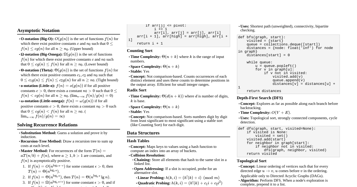
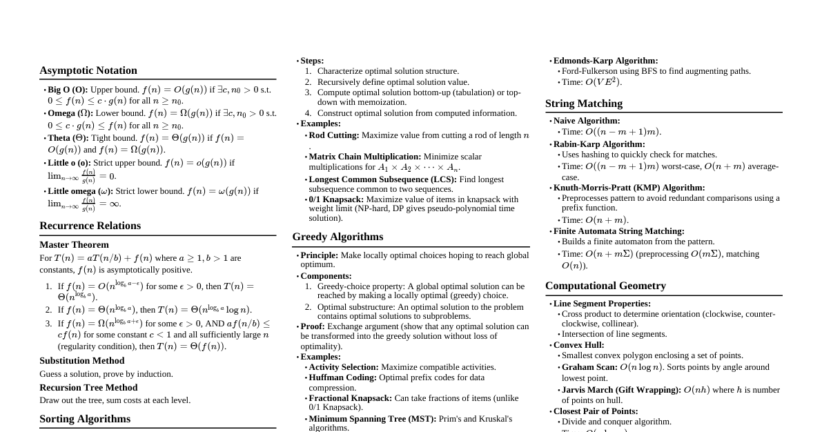
### Asymptotic Notation - **Big O ($O$):** Upper bound. $f(n) = O(g(n))$ if $f(n) \le c \cdot g(n)$ for $n \ge n_0$. - **Omega ($\Omega$):** Lower bound. $f(n) = \Omega(g(n))$ if $f(n) \ge c \cdot g(n)$ for $n \ge n_0$. - **Theta ($\Theta$):** Tight bound. $f(n) = \Theta(g(n))$ if $c_1 \cdot g(n) \le f(n) \le c_2 \cdot g(n)$ for $n \ge n_0$. - **Little o ($o$):** Strict upper bound. $f(n) = o(g(n))$ if $\lim_{n \to \infty} f(n)/g(n) = 0$. - **Little omega ($\omega$):** Strict lower bound. $f(n) = \omega(g(n))$ if $\lim_{n \to \infty} f(n)/g(n) = \infty$. ### Recurrence Relations - **Substitution Method:** Guess a bound and use induction to prove it. - **Recursion-Tree Method:** Draw a tree, sum costs per level, sum costs across levels. - **Master Theorem:** For $T(n) = aT(n/b) + f(n)$: 1. If $f(n) = O(n^{\log_b a - \epsilon})$ for $\epsilon > 0$, then $T(n) = \Theta(n^{\log_b a})$. 2. If $f(n) = \Theta(n^{\log_b a})$, then $T(n) = \Theta(n^{\log_b a} \log n)$. 3. If $f(n) = \Omega(n^{\log_b a + \epsilon})$ for $\epsilon > 0$ and $af(n/b) \le cf(n)$ for some $c ### Sorting Algorithms #### Insertion Sort - **Idea:** Build sorted array one item at a time. - **Time:** $O(n^2)$ worst-case, $O(n)$ best-case (nearly sorted). - **Space:** $O(1)$ in-place. #### Merge Sort - **Idea:** Divide array into halves, sort each half, merge sorted halves. - **Recurrence:** $T(n) = 2T(n/2) + \Theta(n)$. - **Time:** $O(n \log n)$ always. - **Space:** $O(n)$ for merging. #### Heap Sort - **Idea:** Use a max-heap. Build heap, then repeatedly extract max and rebuild heap. - **Time:** $O(n \log n)$ always (build heap $O(n)$, $n$ extracts $O(\log n)$ each). - **Space:** $O(1)$ in-place. #### Quick Sort - **Idea:** Divide and conquer. Pick a pivot, partition array around pivot. Recursively sort sub-arrays. - **Time:** $O(n \log n)$ average, $O(n^2)$ worst-case (unbalanced partitions). - **Space:** $O(\log n)$ average (recursion stack), $O(n)$ worst-case. - **Randomized Quick Sort:** Pick pivot randomly to achieve $O(n \log n)$ expected time. #### Counting Sort - **Idea:** For integers in a small range $[0, k]$. Count occurrences of each number. - **Time:** $O(n+k)$. - **Space:** $O(k)$. - **Stable:** Yes. #### Radix Sort - **Idea:** Sorts numbers by processing digits from least significant to most significant (LSD radix sort) using a stable sort (like Counting Sort). - **Time:** $O(d(n+k))$ where $d$ is number of digits, $k$ is range of digits. ### Data Structures #### Hash Tables - **Direct Addressing:** Array $A$ where $A[k]$ stores element with key $k$. $O(1)$ operations, but requires small key range. - **Collision Resolution:** - **Chaining:** Each slot stores a linked list of elements. Average $O(1+\alpha)$ for operations, where $\alpha=n/m$ (load factor). - **Open Addressing:** All elements in table itself. - **Linear Probing:** $h(k, i) = (h'(k) + i) \pmod m$. Suffers from primary clustering. - **Quadratic Probing:** $h(k, i) = (h'(k) + c_1i + c_2i^2) \pmod m$. Suffers from secondary clustering. - **Double Hashing:** $h(k, i) = (h_1(k) + i \cdot h_2(k)) \pmod m$. Best performance. - **Universal Hashing:** Choose hash function randomly from a family of functions to avoid worst-case behavior. #### Binary Search Trees (BST) - **Property:** For any node $x$, all keys in left subtree $\le \text{key}[x]$, all keys in right subtree $\ge \text{key}[x]$. - **Operations:** Search, Min, Max, Successor, Predecessor, Insert, Delete. Average $O(h)$ where $h$ is height. - **Worst-case:** $O(n)$ for skewed tree. #### Red-Black Trees - **Self-balancing BST:** Guarantees height $O(\log n)$. - **Properties:** 1. Node is Red or Black. 2. Root is Black. 3. Leaves (NIL) are Black. 4. If node is Red, its children are Black. 5. All paths from node to descendant NIL leaves have same number of Black nodes (black-height). - **Operations:** Search $O(\log n)$, Insert $O(\log n)$, Delete $O(\log n)$. #### B-Trees - **Optimized for disk access:** Nodes can have many children ($t$ to $2t$ children, where $t$ is min degree). - **Height:** $O(\log_t n)$. - **Operations:** Search, Insert, Delete $O(t \log_t n)$ disk accesses. #### Fibonacci Heaps - **Amortized analysis:** - **Operations:** - `MAKE-HEAP`: $O(1)$ - `INSERT`: $O(1)$ - `MINIMUM`: $O(1)$ - `EXTRACT-MIN`: $O(\log n)$ amortized - `DECREASE-KEY`: $O(1)$ amortized - `DELETE`: $O(\log n)$ amortized - `UNION`: $O(1)$ ### Dynamic Programming - **Characteristics:** Optimal substructure, overlapping subproblems. - **Steps:** 1. Characterize optimal solution structure. 2. Recursively define optimal solution value. 3. Compute value bottom-up (tabulation) or top-down with memoization. 4. Construct optimal solution (optional). - **Examples:** - **Rod Cutting:** Maximize revenue by cutting rod into pieces. - **Matrix Chain Multiplication:** Find optimal parenthesization to minimize scalar multiplications. - **Longest Common Subsequence (LCS):** Find longest subsequence common to two sequences. - **0/1 Knapsack:** Maximize value of items in knapsack with weight limit (NP-hard, DP gives pseudo-polynomial solution). ### Greedy Algorithms - **Characteristics:** Optimal substructure, greedy choice property (locally optimal choice leads to globally optimal solution). - **Steps:** 1. Cast optimization problem as one where making a choice creates a subproblem. 2. Prove greedy choice property holds. 3. Prove optimal substructure property holds. 4. Construct recursive solution. 5. Convert to iterative solution. - **Examples:** - **Activity Selection:** Select max number of non-overlapping activities. - **Huffman Coding:** Construct optimal prefix codes for data compression. - **Fractional Knapsack:** Maximize value of items, can take fractions (unlike 0/1 Knapsack). ### Graph Algorithms #### Graph Representations - **Adjacency Matrix:** $A[i][j]=1$ if edge $(i,j)$ exists. $O(V^2)$ space. Good for dense graphs. - **Adjacency List:** Array of lists, $Adj[u]$ contains neighbors of $u$. $O(V+E)$ space. Good for sparse graphs. #### Breadth-First Search (BFS) - **Idea:** Explore graph layer by layer from source. Uses a queue. - **Time:** $O(V+E)$. - **Applications:** Shortest path in unweighted graphs, finding connected components. #### Depth-First Search (DFS) - **Idea:** Explore as far as possible along each branch before backtracking. Uses a stack (or recursion). - **Time:** $O(V+E)$. - **Applications:** Topological sort, strongly connected components, cycle detection. #### Topological Sort - **Idea:** Linear ordering of vertices such that for every directed edge $(u,v)$, $u$ comes before $v$. Only for DAGs. - **Method:** Run DFS, order vertices by decreasing finish times. - **Time:** $O(V+E)$. #### Minimum Spanning Trees (MST) - **Goal:** Find a subset of edges that connects all vertices with minimum total edge weight. - **Properties:** Cut property, cycle property. - **Prim's Algorithm:** Grow MST from a starting vertex using a min-priority queue. - **Time:** $O(E \log V)$ with binary heap, $O(E + V \log V)$ with Fibonacci heap. - **Kruskal's Algorithm:** Sort edges by weight, add edges if they don't form a cycle using a Disjoint-Set data structure. - **Time:** $O(E \log E)$ or $O(E \log V)$. #### Single-Source Shortest Paths - **Bellman-Ford Algorithm:** For graphs with negative edge weights. Detects negative cycles. - **Time:** $O(VE)$. - **Output:** true if no negative cycles, false otherwise; shortest paths from source. - **Dijkstra's Algorithm:** For graphs with non-negative edge weights. Uses a min-priority queue. - **Time:** $O(E \log V)$ with binary heap, $O(E + V \log V)$ with Fibonacci heap. - **DAG Shortest Paths:** For Directed Acyclic Graphs. - **Method:** Topologically sort vertices, then relax edges in topological order. - **Time:** $O(V+E)$. #### All-Pairs Shortest Paths - **Floyd-Warshall Algorithm:** DP approach. Computes shortest paths between all pairs of vertices. - **Time:** $O(V^3)$. - **Can handle negative edge weights (but not negative cycles).** - **Johnson's Algorithm:** Re-weights edges using Bellman-Ford, then runs Dijkstra from each vertex. - **Time:** $O(VE + V^2 \log V)$. - **Better than Floyd-Warshall for sparse graphs.** #### Maximum Flow - **Ford-Fulkerson Method:** Finds max flow in a flow network. Uses augmenting paths. - **Time:** Depends on specific augmenting path strategy (e.g., Edmonds-Karp is $O(VE^2)$). - **Max-Flow Min-Cut Theorem:** Max flow value from source to sink equals min capacity of an s-t cut. ### String Matching - **Naive Algorithm:** Shifts pattern one position at a time. $O((n-m+1)m)$. - **Rabin-Karp Algorithm:** Uses hashing to quickly check for matches. - **Time:** $O(n+m)$ average, $O(nm)$ worst-case (spurious hits). - **Knuth-Morris-Pratt (KMP) Algorithm:** Uses a precomputed prefix function to avoid re-matching characters. - **Time:** $O(n+m)$. - **Finite Automata:** Construct a finite automaton for pattern. - **Time:** Preprocessing $O(m |\Sigma|)$, Matching $O(n)$. ### Computational Geometry - **Line Segment Properties:** - **Cross Product:** Determines orientation of three points (clockwise, counter-clockwise, collinear). - **Intersection:** Check if two segments intersect. - **Convex Hull:** Smallest convex polygon enclosing a set of points. - **Graham Scan:** Sort points by angle, use stack to maintain convex hull. $O(n \log n)$. - **Jarvis March (Gift Wrapping):** Find extreme point, then repeatedly find next point with smallest polar angle. $O(nh)$, where $h$ is number of points on hull. ### NP-Completeness - **P (Polynomial Time):** Problems solvable in polynomial time. - **NP (Nondeterministic Polynomial Time):** Problems whose solutions can be verified in polynomial time. - **NP-Hard:** Problems to which all NP problems can be reduced in polynomial time. - **NP-Complete (NPC):** Problems that are in NP and are NP-Hard. - **Reductions:** If $L_1 \le_P L_2$ (read $L_1$ reduces to $L_2$ in polynomial time), then: - If $L_2 \in P$, then $L_1 \in P$. - If $L_1$ is NP-Hard, then $L_2$ is NP-Hard. - **Common NPC Problems:** SAT, 3-SAT, Clique, Vertex Cover, Hamiltonian Cycle, Traveling Salesperson Problem, Subset Sum, Knapsack.