Quadratic Equations Compendium

Cheatsheet Content

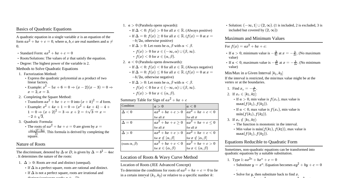
### Introduction to Quadratic Equations A quadratic equation is a polynomial equation of the second degree. The general form is: $$ax^2 + bx + c = 0$$ where $a, b, c$ are real numbers and $a \neq 0$. Quadratic equations are fundamental in mathematics, physics, engineering, and economics, appearing in diverse applications from projectile motion to optimization problems. Understanding their properties and solution methods is crucial for higher studies. ### Standard Form and Terminology - **Standard Form:** $ax^2 + bx + c = 0$ - **Coefficients:** - $a$: leading coefficient (coefficient of $x^2$) - $b$: linear coefficient (coefficient of $x$) - $c$: constant term - **Roots/Solutions:** The values of $x$ that satisfy the equation. A quadratic equation always has two roots, which may be real or complex, and distinct or repeated. - **Parabola:** The graph of a quadratic function $y = ax^2 + bx + c$ is a parabola. The roots of the equation correspond to the x-intercepts of the parabola. ### Methods of Solving Quadratic Equations #### 1. Factoring This method is applicable when the quadratic expression can be factored into two linear factors. If $ax^2 + bx + c = (px + q)(rx + s) = 0$, then $x = -q/p$ or $x = -s/r$. **Example:** Solve $x^2 - 5x + 6 = 0$ $(x - 2)(x - 3) = 0$ $x - 2 = 0 \implies x = 2$ $x - 3 = 0 \implies x = 3$ #### 2. Using the Quadratic Formula The most general method, always yields the roots. $$x = \frac{-b \pm \sqrt{b^2 - 4ac}}{2a}$$ **Derivation (Completing the Square):** $ax^2 + bx + c = 0$ $ax^2 + bx = -c$ $x^2 + \frac{b}{a}x = -\frac{c}{a}$ $x^2 + \frac{b}{a}x + \left(\frac{b}{2a}\right)^2 = -\frac{c}{a} + \left(\frac{b}{2a}\right)^2$ $\left(x + \frac{b}{2a}\right)^2 = \frac{b^2 - 4ac}{4a^2}$ $x + \frac{b}{2a} = \pm \sqrt{\frac{b^2 - 4ac}{4a^2}}$ $x = -\frac{b}{2a} \pm \frac{\sqrt{b^2 - 4ac}}{2a}$ $x = \frac{-b \pm \sqrt{b^2 - 4ac}}{2a}$ #### 3. Completing the Square Useful for deriving the quadratic formula and for transforming quadratic functions into vertex form. **Example:** Solve $x^2 + 6x + 5 = 0$ $x^2 + 6x = -5$ $x^2 + 6x + (6/2)^2 = -5 + (6/2)^2$ $x^2 + 6x + 9 = -5 + 9$ $(x + 3)^2 = 4$ $x + 3 = \pm\sqrt{4}$ $x + 3 = \pm 2$ $x = -3 \pm 2$ $x_1 = -1, x_2 = -5$ #### 4. Graphing The roots are the x-intercepts of the parabola $y = ax^2 + bx + c$. This method gives approximate solutions and is good for visualization. ### The Discriminant ($\Delta$) The term $b^2 - 4ac$ from the quadratic formula is called the discriminant, denoted by $\Delta$. It determines the nature of the roots. - If $\Delta > 0$: Two distinct real roots. The parabola intersects the x-axis at two different points. - If $\Delta = 0$: One real root (a repeated or double root). The parabola touches the x-axis at exactly one point (its vertex). - If $\Delta ### Properties of Roots (Vieta's Formulas) For a quadratic equation $ax^2 + bx + c = 0$ with roots $x_1$ and $x_2$: - **Sum of roots:** $x_1 + x_2 = -\frac{b}{a}$ - **Product of roots:** $x_1 x_2 = \frac{c}{a}$ These formulas are extremely useful for forming quadratic equations given their roots, or for finding relationships between roots without explicitly solving the equation. **Example:** If the roots of $2x^2 - 8x + 6 = 0$ are $\alpha$ and $\beta$, find $\alpha + \beta$ and $\alpha\beta$. Here $a=2, b=-8, c=6$. $\alpha + \beta = -(-8)/2 = 8/2 = 4$ $\alpha\beta = 6/2 = 3$ (Check: $2x^2 - 8x + 6 = 2(x^2 - 4x + 3) = 2(x-1)(x-3) = 0$. Roots are $x=1, x=3$. Sum $1+3=4$, Product $1 \times 3=3$.) ### Quadratic Functions and Graphs A quadratic function is of the form $f(x) = ax^2 + bx + c$. Its graph is a parabola. - **Vertex Form:** $f(x) = a(x - h)^2 + k$, where $(h, k)$ is the vertex of the parabola. - $h = -\frac{b}{2a}$ - $k = f(h) = a\left(-\frac{b}{2a}\right)^2 + b\left(-\frac{b}{2a}\right) + c = \frac{4ac - b^2}{4a}$ - **Axis of Symmetry:** The vertical line $x = h = -\frac{b}{2a}$. - **Direction of Opening:** - If $a > 0$, the parabola opens upwards (vertex is a minimum point). - If $a ### Applications in Physics #### 1. Projectile Motion The height $h(t)$ of a projectile launched vertically with initial velocity $v_0$ from an initial height $h_0$ is given by: $$h(t) = -\frac{1}{2}gt^2 + v_0t + h_0$$ where $g$ is the acceleration due to gravity ($9.8 \text{ m/s}^2$ or $32 \text{ ft/s}^2$). Finding when the projectile hits the ground means solving $h(t) = 0$ for $t$. Finding the maximum height involves finding the vertex of the parabola. #### 2. Energy Equations Kinetic energy: $KE = \frac{1}{2}mv^2$. If $KE$ is known, velocity $v$ can be found using a quadratic equation. #### 3. Optics (Lens Formula) In some cases, lens equations can lead to quadratic forms when solving for image/object distances or focal lengths. ### Applications in Engineering #### 1. Optimization Problems Minimizing costs or maximizing profits often involves quadratic functions. For example, finding the optimal dimensions for a container to maximize volume or minimize surface area. The vertex of the parabola gives the optimal value. #### 2. Electrical Engineering (RLC Circuits) The transient response of RLC circuits (Resistor-Inductor-Capacitor) is described by second-order differential equations, whose characteristic equations are quadratic. The nature of the roots (real, repeated, complex) determines whether the circuit is overdamped, critically damped, or underdamped. Characteristic equation: $s^2 + \frac{R}{L}s + \frac{1}{LC} = 0$ Roots determine the natural frequencies of the circuit. #### 3. Structural Engineering Calculating stresses, strains, and deflections in beams and other structures can involve quadratic equations, especially when dealing with bending moments and material properties. ### Applications in Economics #### 1. Supply and Demand Equilibrium points in markets can sometimes be found by solving quadratic equations when supply and demand functions are non-linear. #### 2. Profit Maximization If a company's revenue $R(q)$ and cost $C(q)$ functions are given, the profit function $P(q) = R(q) - C(q)$ is often quadratic. Maximizing profit involves finding the vertex of this profit parabola. **Example:** $R(q) = 100q - q^2$, $C(q) = 10q + 50$. $P(q) = (100q - q^2) - (10q + 50) = -q^2 + 90q - 50$. To find maximum profit, find the vertex where $q = -b/(2a) = -90/(2(-1)) = 45$ units. #### 3. Utility Functions In microeconomics, utility functions modeling consumer preferences can sometimes be quadratic, leading to optimization problems solvable with quadratic techniques. ### Quadratic Inequalities A quadratic inequality is an inequality involving a quadratic expression, such as $ax^2 + bx + c > 0$, $ax^2 + bx + c 0$ corresponds to the $x$-values where the parabola $y = ax^2 + bx + c$ is above the x-axis. The solution to $ax^2 + bx + c 0$ 1. Roots of $x^2 - 4x + 3 = 0$ are $(x-1)(x-3) = 0 \implies x=1, x=3$. 2. Intervals: $(-\infty, 1)$, $(1, 3)$, $(3, \infty)$. 3. Test points: - For $(-\infty, 1)$, choose $x=0$: $0^2 - 4(0) + 3 = 3 > 0$ (True) - For $(1, 3)$, choose $x=2$: $2^2 - 4(2) + 3 = 4 - 8 + 3 = -1 > 0$ (False) - For $(3, \infty)$, choose $x=4$: $4^2 - 4(4) + 3 = 16 - 16 + 3 = 3 > 0$ (True) 4. Solution: $(-\infty, 1) \cup (3, \infty)$. ### Simultaneous Equations Involving Quadratics Solving systems where one or both equations are quadratic. **Example:** Solve the system: 1. $y = x^2 - 4$ 2. $y = x - 2$ **Method: Substitution** Substitute (2) into (1): $x - 2 = x^2 - 4$ $0 = x^2 - x - 2$ $0 = (x - 2)(x + 1)$ $x = 2$ or $x = -1$ Substitute $x$ values back into $y = x - 2$: If $x = 2$, $y = 2 - 2 = 0$. Point: $(2, 0)$ If $x = -1$, $y = -1 - 2 = -3$. Point: $(-1, -3)$ These are the intersection points of the parabola $y = x^2 - 4$ and the line $y = x - 2$. ### Higher Degree Equations Reducible to Quadratic Form Some polynomial equations of degree higher than two can be solved by transforming them into a quadratic equation using a substitution. **Form:** $a(x^n)^2 + b(x^n) + c = 0$ or $a(f(x))^2 + b(f(x)) + c = 0$. **Example 1: Biquadratic Equation** Solve $x^4 - 5x^2 + 4 = 0$ Let $u = x^2$. Then the equation becomes: $u^2 - 5u + 4 = 0$ $(u - 1)(u - 4) = 0$ $u = 1$ or $u = 4$ Substitute back $u = x^2$: $x^2 = 1 \implies x = \pm 1$ $x^2 = 4 \implies x = \pm 2$ The four roots are $1, -1, 2, -2$. **Example 2: Exponential Equation** Solve $e^{2x} - 3e^x + 2 = 0$ Let $u = e^x$. Then $e^{2x} = (e^x)^2 = u^2$. $u^2 - 3u + 2 = 0$ $(u - 1)(u - 2) = 0$ $u = 1$ or $u = 2$ Substitute back $u = e^x$: $e^x = 1 \implies x = \ln(1) = 0$ $e^x = 2 \implies x = \ln(2)$ The two roots are $0, \ln(2)$. ### Complex Numbers and Quadratic Equations When the discriminant $\Delta = b^2 - 4ac ### Quadratic Forms in Matrix Algebra A quadratic form is a polynomial where every term has degree two. In $n$ variables $x_1, \ldots, x_n$, it can be written as: $$Q(\mathbf{x}) = \sum_{i=1}^n \sum_{j=1}^n a_{ij}x_i x_j$$ This can be expressed in matrix form as $Q(\mathbf{x}) = \mathbf{x}^T A \mathbf{x}$, where $\mathbf{x}$ is a column vector and $A$ is a symmetric matrix. **Example (2 variables):** $Q(x_1, x_2) = ax_1^2 + 2bx_1x_2 + cx_2^2$ This can be written as: $\begin{pmatrix} x_1 & x_2 \end{pmatrix} \begin{pmatrix} a & b \\ b & c \end{pmatrix} \begin{pmatrix} x_1 \\ x_2 \end{pmatrix}$ Quadratic forms are essential in: - **Optimization:** Determining maxima and minima of functions of several variables (Hessian matrix). - **Geometry:** Describing conic sections (ellipses, hyperbolas, parabolas) and quadric surfaces. - **Statistics:** In multivariate analysis and least squares. - **Physics:** In energy functions and stability analysis. ### Quadratic Regression Quadratic regression is a statistical technique used to find the best-fitting quadratic curve to a set of data points. It is a form of polynomial regression. The model is typically $y = ax^2 + bx + c + \epsilon$, where $\epsilon$ is the error term. **Applications:** - **Modeling non-linear relationships:** When a linear model is not appropriate, a quadratic model can capture curvature in the data. - **Predicting trends:** Useful in forecasting where the trend is expected to accelerate or decelerate. - **Finding optimal points:** If the data suggests a maximum or minimum, quadratic regression can estimate its location. **Method:** Typically solved using least squares, minimizing the sum of squared residuals between the observed data points and the quadratic curve. This involves solving a system of linear equations derived from the partial derivatives of the sum of squares with respect to $a, b, c$. ### Cautions and Common Mistakes - **Incorrectly identifying coefficients:** Ensure the equation is in standard form $ax^2 + bx + c = 0$ before identifying $a, b, c$. - **Sign errors:** Be careful with negative signs, especially in the quadratic formula. - **Dividing by zero:** Remember $a \neq 0$. If $a=0$, it's a linear equation, not quadratic. - **Forgetting $\pm$:** When taking the square root, always include both positive and negative roots. - **Misinterpreting the discriminant:** A negative discriminant means complex roots, not no roots. - **Algebraic errors in completing the square:** Ensure you add the same value to both sides of the equation. - **Complex number arithmetic:** Be precise when dealing with $i = \sqrt{-1}$. ### Summary and Key Takeaways - **General Form:** $ax^2 + bx + c = 0$ - **Quadratic Formula:** $x = \frac{-b \pm \sqrt{b^2 - 4ac}}{2a}$ - **Discriminant ($\Delta = b^2 - 4ac$):** Determines the nature of the roots (real/complex, distinct/repeated). - **Vieta's Formulas:** $x_1 + x_2 = -b/a$, $x_1 x_2 = c/a$. - **Vertex Form:** $f(x) = a(x - h)^2 + k$, vertex at $(h,k)$. - **Applications:** Ubiquitous in physics (projectile motion), engineering (circuits, optimization), economics (profit maximization), and statistics (regression). - **Inequalities:** Solved by finding critical points and testing intervals or using graphical interpretation. - **Reducible Forms:** Higher-degree equations can often be transformed into quadratics via substitution. - **Complex Roots:** Occur when $\Delta