Introduction to Algorithms (CLRS)

Cheatsheet Content

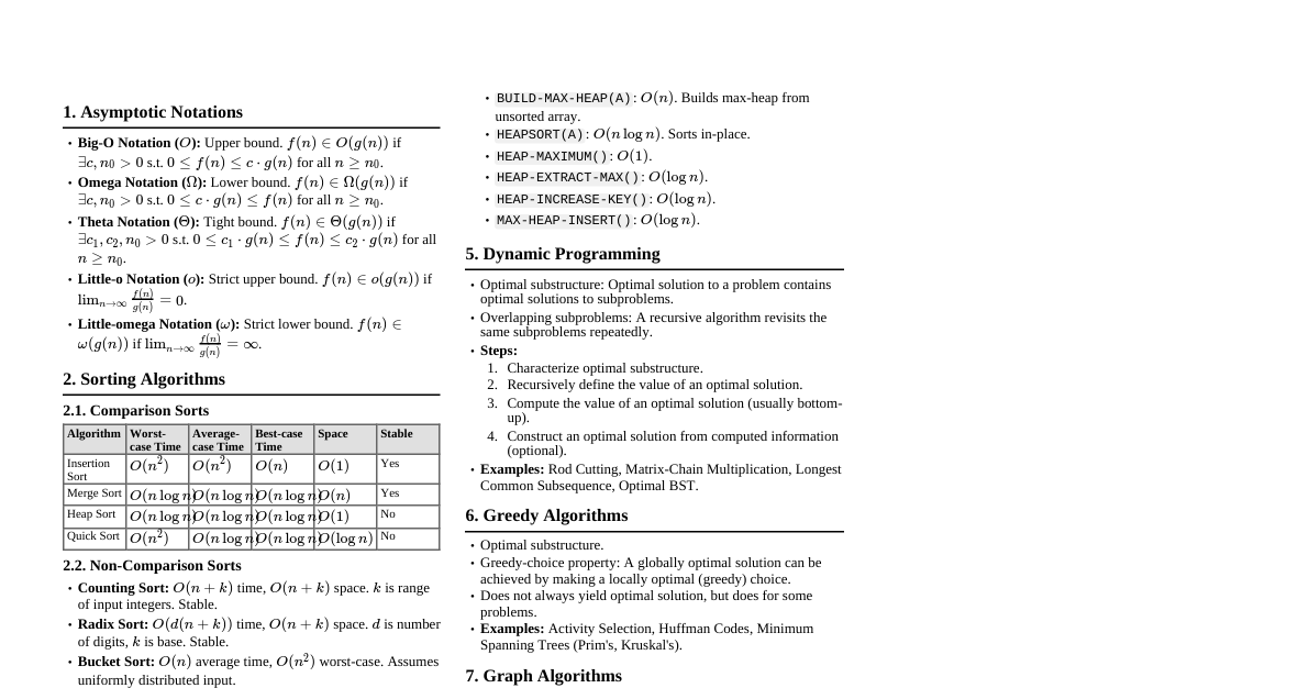
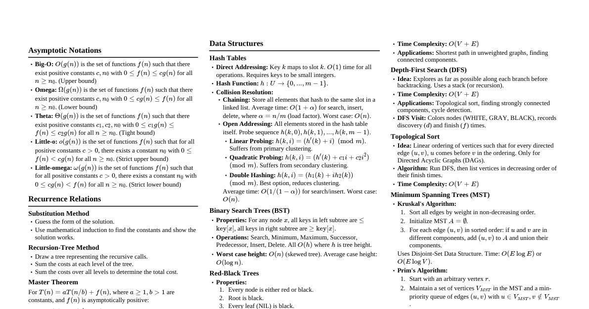
Asymptotic Notations Big-O Notation: $O(g(n))$ - Upper bound. $f(n) = O(g(n))$ if there exist positive constants $c, n_0$ such that $0 \le f(n) \le c g(n)$ for all $n \ge n_0$. Omega Notation: $\Omega(g(n))$ - Lower bound. $f(n) = \Omega(g(n))$ if there exist positive constants $c, n_0$ such that $0 \le c g(n) \le f(n)$ for all $n \ge n_0$. Theta Notation: $\Theta(g(n))$ - Tight bound. $f(n) = \Theta(g(n))$ if there exist positive constants $c_1, c_2, n_0$ such that $0 \le c_1 g(n) \le f(n) \le c_2 g(n)$ for all $n \ge n_0$. Little-o Notation: $o(g(n))$ - Strict upper bound. $f(n) = o(g(n))$ if for all positive constants $c > 0$, there exists an $n_0$ such that $0 \le f(n) Little-omega Notation: $\omega(g(n))$ - Strict lower bound. $f(n) = \omega(g(n))$ if for all positive constants $c > 0$, there exists an $n_0$ such that $0 \le c g(n) Solving Recurrences 1. Substitution Method Guess the form of the solution. Use mathematical induction to find constants and show the solution works. Example: $T(n) = 2T(\lfloor n/2 \rfloor) + n$. Guess $T(n) = O(n \log n)$. Assume $T(k) \le c k \log k$ for $k $T(n) \le 2(c \lfloor n/2 \rfloor \log(\lfloor n/2 \rfloor)) + n \le 2(c (n/2) \log(n/2)) + n = cn \log n - cn + n \le cn \log n$ for $c \ge 1$. 2. Recursion-Tree Method Draw a recursion tree illustrating the costs at each level of recursion. Sum the costs at each level to get the total cost. Example: $T(n) = 3T(n/4) + cn^2$. Level 0: $cn^2$ Level 1: $3c(n/4)^2 = 3cn^2/16$ Level 2: $3^2c(n/16)^2 = 9cn^2/256$ Total cost per level: $(3/16)^i cn^2$ Sum: $cn^2 \sum_{i=0}^{\log_4 n - 1} (3/16)^i = cn^2 \frac{1 - (3/16)^{\log_4 n}}{1 - 3/16} = cn^2 \frac{1 - n^{\log_4(3/16)}}{13/16} = O(n^2)$. 3. Master Method For recurrences of the form $T(n) = aT(n/b) + f(n)$, where $a \ge 1, b > 1, f(n)$ is asymptotically positive. Case 1: If $f(n) = O(n^{\log_b a - \epsilon})$ for some constant $\epsilon > 0$, then $T(n) = \Theta(n^{\log_b a})$. Case 2: If $f(n) = \Theta(n^{\log_b a})$, then $T(n) = \Theta(n^{\log_b a} \log n)$. Case 3: If $f(n) = \Omega(n^{\log_b a + \epsilon})$ for some constant $\epsilon > 0$, AND if $af(n/b) \le c f(n)$ for some constant $c Sorting Algorithms Algorithm Worst-case Time Avg-case Time Best-case Time Space Stable Insertion Sort $O(n^2)$ $O(n^2)$ $O(n)$ $O(1)$ Yes Merge Sort $O(n \log n)$ $O(n \log n)$ $O(n \log n)$ $O(n)$ Yes Heap Sort $O(n \log n)$ $O(n \log n)$ $O(n \log n)$ $O(1)$ No Quick Sort $O(n^2)$ $O(n \log n)$ $O(n \log n)$ $O(\log n)$ No Counting Sort $O(n+k)$ $O(n+k)$ $O(n+k)$ $O(n+k)$ Yes Radix Sort $O(d(n+k))$ $O(d(n+k))$ $O(d(n+k))$ $O(n+k)$ Yes Comparison Sort Lower Bound: Any comparison sort algorithm requires $\Omega(n \log n)$ comparisons in the worst case. Data Structures Hash Tables Direct-Address Tables: $O(1)$ for all operations, but requires key range to be small. Collision Resolution: Chaining: Each slot stores a linked list of elements. Avg-case $O(1+\alpha)$, worst-case $O(n)$ where $\alpha = n/m$ (load factor). Open Addressing: All elements stored in table itself. Linear probing: $h(k, i) = (h'(k) + i) \pmod m$ Quadratic probing: $h(k, i) = (h'(k) + c_1 i + c_2 i^2) \pmod m$ Double hashing: $h(k, i) = (h_1(k) + i h_2(k)) \pmod m$ Avg-case $O(1/(1-\alpha))$, worst-case $O(n)$. Binary Search Trees (BST) Operations (Search, Min, Max, Successor, Predecessor, Insert, Delete): $O(h)$ where $h$ is the height of the tree. Worst-case height: $O(n)$ (skewed tree). Red-Black Trees Self-balancing BST. Height $O(\log n)$. Operations: $O(\log n)$ for Search, Insert, Delete. Properties: Every node is red or black. Root is black. Every leaf (NIL) is black. If a node is red, both its children are black. All simple paths from a node to any descendant leaf contain the same number of black nodes (black-height). Dynamic Programming Optimal substructure and overlapping subproblems. Steps: Characterize optimal substructure. Recursively define the value of an optimal solution. Compute the value of an optimal solution bottom-up (tabulation) or top-down with memoization. Construct an optimal solution from computed information. Examples: Longest Common Subsequence (LCS) Matrix Chain Multiplication Rod Cutting Graph Algorithms Representations Adjacency List: $O(V+E)$ space. Good for sparse graphs. Adjacency Matrix: $O(V^2)$ space. Good for dense graphs. Breadth-First Search (BFS) Explores graph level by level. Time: $O(V+E)$ for adjacency list. Finds shortest paths in unweighted graphs. Depth-First Search (DFS) Explores as far as possible along each branch before backtracking. Time: $O(V+E)$ for adjacency list. Used for topological sort, strongly connected components. Minimum Spanning Trees (MST) Prim's Algorithm: Grows a single tree. Uses a min-priority queue. Time: $O(E \log V)$ with binary heap, $O(E + V \log V)$ with Fibonacci heap. Kruskal's Algorithm: Adds edges in increasing order of weight, avoiding cycles. Uses Disjoint Set Union. Time: $O(E \log E)$ or $O(E \log V)$. Shortest Paths Dijkstra's Algorithm: For single-source shortest paths with non-negative edge weights. Uses a min-priority queue. Time: $O(E \log V)$ with binary heap, $O(E + V \log V)$ with Fibonacci heap. Bellman-Ford Algorithm: For single-source shortest paths, allows negative edge weights. Detects negative cycles. Time: $O(VE)$. Floyd-Warshall Algorithm: For all-pairs shortest paths. Uses dynamic programming. Time: $O(V^3)$. Johnson's Algorithm: For all-pairs shortest paths on sparse graphs, can handle negative weights. Re-weights graph using Bellman-Ford, then runs Dijkstra $V$ times. Time: $O(V E \log V)$ with binary heap, $O(V^2 \log V + VE)$ with Fibonacci heap. Greedy Algorithms Makes locally optimal choices in the hope of finding a global optimum. Properties: Greedy-choice property: A globally optimal solution can be reached by making a locally optimal (greedy) choice. Optimal substructure: An optimal solution to the problem contains optimal solutions to subproblems. Examples: Activity Selection Problem Huffman Coding Fractional Knapsack Problem Prim's and Kruskal's MST algorithms Dijkstra's algorithm Complexity Classes P: Problems solvable in polynomial time by a deterministic Turing machine. NP: Problems verifiable in polynomial time by a deterministic Turing machine (or solvable in polynomial time by a non-deterministic Turing machine). NP-Complete (NPC): Problems in NP such that every problem in NP can be reduced to them in polynomial time. If an NPC problem can be solved in polynomial time, then P = NP. NP-Hard: Problems to which every problem in NP can be reduced in polynomial time. (Does not necessarily have to be in NP itself). Common NP-Complete Problems 3-SAT Clique Vertex Cover Hamiltonian Cycle Traveling Salesperson Problem (TSP) Subset Sum Knapsack Problem (0/1) Amortized Analysis A method for analyzing a sequence of operations to determine the average cost per operation. Methods: Aggregate Analysis: Compute total cost of $n$ operations, then divide by $n$. Accounting Method: Assign "credits" to operations. Overcharge some operations, use credits for others. Total credits in data structure should not be negative. Potential Method: Define a potential function $\Phi$ that maps states of the data structure to real numbers. Amortized cost: $\hat{c_i} = c_i + \Phi(D_i) - \Phi(D_{i-1})$. Example: Dynamic Array (amortized $O(1)$ for append).