Introduction to Algorithms (CLRS)

Cheatsheet Content

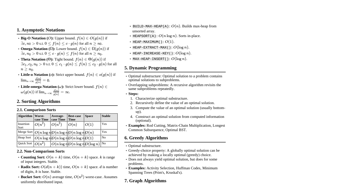
1. Asymptotic Notations Big-O Notation: $O(g(n)) = \{f(n) : \exists c, n_0 > 0 \text{ s.t. } 0 \le f(n) \le c \cdot g(n) \text{ for all } n \ge n_0\}$ Omega Notation: $\Omega(g(n)) = \{f(n) : \exists c, n_0 > 0 \text{ s.t. } 0 \le c \cdot g(n) \le f(n) \text{ for all } n \ge n_0\}$ Theta Notation: $\Theta(g(n)) = \{f(n) : \exists c_1, c_2, n_0 > 0 \text{ s.t. } 0 \le c_1 \cdot g(n) \le f(n) \le c_2 \cdot g(n) \text{ for all } n \ge n_0\}$ Little-o Notation: $o(g(n)) = \{f(n) : \forall c > 0, \exists n_0 > 0 \text{ s.t. } 0 \le f(n) Little-omega Notation: $\omega(g(n)) = \{f(n) : \forall c > 0, \exists n_0 > 0 \text{ s.t. } 0 \le c \cdot g(n) 2. Recurrence Relations 2.1. Master Theorem: $T(n) = aT(n/b) + f(n)$ Case 1: If $f(n) = O(n^{\log_b a - \epsilon})$ for some $\epsilon > 0$, then $T(n) = \Theta(n^{\log_b a})$. Case 2: If $f(n) = \Theta(n^{\log_b a} \log^k n)$ for some $k \ge 0$, then $T(n) = \Theta(n^{\log_b a} \log^{k+1} n)$. Case 3: If $f(n) = \Omega(n^{\log_b a + \epsilon})$ for some $\epsilon > 0$, AND $af(n/b) \le cf(n)$ for some $c 2.2. Substitution Method Guess the form of the solution. Use mathematical induction to find constants and show the solution works. 2.3. Recursion-Tree Method Draw a tree showing costs at each level of recursion. Sum costs across levels to get total. Useful for generating good guesses for substitution method. 3. Sorting Algorithms Algorithm Time Complexity (Avg) Time Complexity (Worst) Space Complexity Stable Insertion Sort $\Theta(n^2)$ $O(n^2)$ $O(1)$ Yes Merge Sort $\Theta(n \log n)$ $O(n \log n)$ $O(n)$ Yes Heapsort $\Theta(n \log n)$ $O(n \log n)$ $O(1)$ No Quicksort $\Theta(n \log n)$ $O(n^2)$ $O(\log n)$ (Avg) No Counting Sort $\Theta(n+k)$ $O(n+k)$ $O(n+k)$ Yes Radix Sort $\Theta(d(n+k))$ $O(d(n+k))$ $O(n+k)$ Yes 3.1. Lower Bound for Comparison Sorts Comparison sorts require $\Omega(n \log n)$ comparisons in the worst case. 4. Data Structures 4.1. Hash Tables Direct Addressing: $O(1)$ for all ops, but needs array of size $U$ (universe). Chaining: Linked list for collisions. Avg $O(1+\alpha)$ for search, insert, delete, where $\alpha=n/m$ (load factor). Worst $O(n)$. Open Addressing: Probing for empty slot. Linear Probing: $h(k, i) = (h'(k) + i) \pmod m$ Quadratic Probing: $h(k, i) = (h'(k) + c_1i + c_2i^2) \pmod m$ Double Hashing: $h(k, i) = (h_1(k) + i \cdot h_2(k)) \pmod m$ Universal Hashing: Probabilistically guarantees good average-case performance. 4.2. Binary Search Trees (BST) Search, Min, Max, Successor, Predecessor, Insert, Delete: $O(h)$ where $h$ is height. Worst case $h=O(n)$, best case $h=O(\log n)$. 4.3. Red-Black Trees Self-balancing BST. Height $h = O(\log n)$. All basic operations (search, insert, delete) take $O(\log n)$ time. Properties: Every node is Red or Black. Root is Black. Every leaf (NIL) is Black. If a node is Red, its children are Black. All simple paths from node to descendant leaf contain same number of Black nodes. 4.4. Augmenting Data Structures Add additional information to nodes (e.g., size in order-statistic trees). Maintain info during modifications without affecting asymptotic running times. 5. Dynamic Programming Optimal substructure: Optimal solution to a problem contains optimal solutions to subproblems. Overlapping subproblems: A recursive algorithm revisits the same subproblems repeatedly. Steps: Characterize optimal substructure. Recursively define the value of an optimal solution. Compute the value of an optimal solution (bottom-up or memoized). Construct an optimal solution from computed information. Examples: Rod Cutting, Matrix-Chain Multiplication, Longest Common Subsequence, Optimal BST. 6. Greedy Algorithms Make locally optimal choices in the hope that they lead to a globally optimal solution. Properties: Greedy choice property: A globally optimal solution can be arrived at by making a locally optimal (greedy) choice. Optimal substructure: An optimal solution to the problem contains optimal solutions to subproblems. Examples: Activity Selection, Huffman Codes, Fractional Knapsack. 7. Graph Algorithms 7.1. Graph Representations Adjacency List: $V$ lists, total $O(V+E)$ space. Good for sparse graphs. Adjacency Matrix: $V \times V$ matrix, $O(V^2)$ space. Good for dense graphs. 7.2. Breadth-First Search (BFS) Explores graph level by level. Finds shortest path in terms of number of edges for unweighted graphs. Time: $O(V+E)$. 7.3. Depth-First Search (DFS) Explores as far as possible along each branch before backtracking. Discovers paths, cycles, topological sorts. Time: $O(V+E)$. 7.4. Topological Sort Linear ordering of vertices such that for every directed edge $(u, v)$, $u$ comes before $v$. Applicable only to Directed Acyclic Graphs (DAGs). Time: $O(V+E)$ (using DFS). 7.5. Minimum Spanning Trees (MST) Connects all vertices with minimum total edge weight. Prim's Algorithm: Grows a single tree. Uses a min-priority queue. Time: $O(E \log V)$ or $O(E + V \log V)$ with Fibonacci heap. Kruskal's Algorithm: Adds edges in increasing order of weight, avoiding cycles. Uses Disjoint-Set Union. Time: $O(E \log E)$ or $O(E \log V)$. 7.6. Single-Source Shortest Paths Bellman-Ford Algorithm: Handles negative edge weights. Detects negative cycles. Time: $O(VE)$. Dijkstra's Algorithm: Non-negative edge weights only. Uses a min-priority queue. Time: $O(E \log V)$ or $O(E + V \log V)$ with Fibonacci heap. DAG Shortest Paths: Relax edges in topological sort order. Time: $O(V+E)$. 7.7. All-Pairs Shortest Paths Floyd-Warshall Algorithm: Dynamic programming. Time: $O(V^3)$. Johnson's Algorithm: Sparse graphs with negative weights. Reweights edges using Bellman-Ford, then $V$ Dijkstra runs. Time: $O(VE + V^2 \log V)$. 7.8. Maximum Flow Ford-Fulkerson Method: Finds augmenting paths in residual graph. Time depends on path finding and capacities. Edmonds-Karp: Uses BFS to find augmenting paths. Time: $O(VE^2)$. 8. String Matching Naive Algorithm: $O((n-m+1)m)$. Rabin-Karp Algorithm: Uses hashing. Average $O(n+m)$, worst $O((n-m+1)m)$. Knuth-Morris-Pratt (KMP) Algorithm: Uses a prefix function to avoid redundant comparisons. Time: $O(n+m)$. 9. NP-Completeness P: Class of problems solvable in polynomial time. NP: Class of problems whose solutions can be verified in polynomial time. NP-Hard: A problem $H$ is NP-hard if for every problem $L \in NP$, $L \le_P H$ (L is polynomial-time reducible to H). NP-Complete: A problem $C$ is NP-complete if $C \in NP$ and $C$ is NP-hard. Common NP-Complete Problems: Satisfiability (SAT) 3-CNF Satisfiability (3-SAT) Clique Vertex Cover Hamiltonian Cycle Traveling Salesperson Problem (TSP) Subset Sum Knapsack 10. Amortized Analysis Averages the time required to perform a sequence of operations. Methods: Aggregate Analysis: Total cost for $n$ operations / $n$. Accounting Method: Assigns "credit" to operations, pays for future expensive operations. Potential Method: Uses a potential function $\Phi$ to smooth out costs. $c_i' = c_i + \Phi(D_i) - \Phi(D_{i-1})$. Examples: Dynamic Array (doubling), Multi-pop stack.