Introduction to Algorithms (CLRS)

Cheatsheet Content

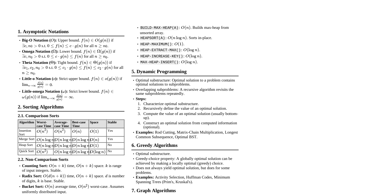
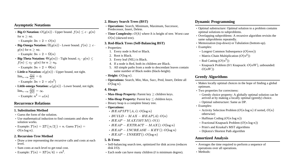
Asymptotic Notations Big O: $O(g(n))$ is the set of functions $f(n)$ such that there exist positive constants $c, n_0$ with $0 \le f(n) \le c g(n)$ for all $n \ge n_0$. (Upper bound) Omega: $\Omega(g(n))$ is the set of functions $f(n)$ such that there exist positive constants $c, n_0$ with $0 \le c g(n) \le f(n)$ for all $n \ge n_0$. (Lower bound) Theta: $\Theta(g(n))$ is the set of functions $f(n)$ such that there exist positive constants $c_1, c_2, n_0$ with $0 \le c_1 g(n) \le f(n) \le c_2 g(n)$ for all $n \ge n_0$. (Tight bound) Little o: $o(g(n))$ is the set of functions $f(n)$ such that for any positive constant $c > 0$, there exists a constant $n_0$ with $0 \le f(n) Little omega: $\omega(g(n))$ is the set of functions $f(n)$ such that for any positive constant $c > 0$, there exists a constant $n_0$ with $0 \le c g(n) Solving Recurrences 1. Substitution Method Guess the form of the solution. Use mathematical induction to find the constants and show the solution works. 2. Recursion-Tree Method Draw a recursion tree to visualize the costs at each level of recursion. Sum the costs at all levels to determine the total cost. Useful for generating good guesses for the substitution method. 3. Master Method For recurrences of the form $T(n) = a T(n/b) + f(n)$, where $a \ge 1, b > 1$ are constants, and $f(n)$ is an asymptotically positive function. If $f(n) = O(n^{\log_b a - \epsilon})$ for some constant $\epsilon > 0$, then $T(n) = \Theta(n^{\log_b a})$. If $f(n) = \Theta(n^{\log_b a})$, then $T(n) = \Theta(n^{\log_b a} \log n)$. If $f(n) = \Omega(n^{\log_b a + \epsilon})$ for some constant $\epsilon > 0$, AND $a f(n/b) \le c f(n)$ for some constant $c Sorting Algorithms 1. Insertion Sort Time Complexity: $O(n^2)$ worst-case, $O(n)$ best-case. Space Complexity: $O(1)$. Stable: Yes. In-place: Yes. Concept: Builds the final sorted array one item at a time. Iterates through input elements and inserts each into its correct position in the sorted part. 2. Merge Sort Time Complexity: $\Theta(n \log n)$ in all cases. Recurrence: $T(n) = 2T(n/2) + \Theta(n)$. Space Complexity: $O(n)$ (for temporary arrays). Stable: Yes. In-place: No. Concept: Divide and Conquer. Divides unsorted list into $n$ sublists, each containing one element, then repeatedly merges sublists to produce new sorted sublists until there is only one sublist remaining. 3. Heap Sort Time Complexity: $\Theta(n \log n)$ in all cases. Space Complexity: $O(1)$ (in-place). Stable: No. In-place: Yes. Concept: Builds a max-heap from the input data, then repeatedly extracts the maximum element and rebuilds the heap. Build-Max-Heap: $O(n)$. Heapify: $O(\log n)$. 4. Quick Sort Time Complexity: $O(n \log n)$ average-case, $O(n^2)$ worst-case. Space Complexity: $O(\log n)$ average-case (for recursion stack), $O(n)$ worst-case. Stable: No. In-place: Yes (partitioning). Concept: Divide and Conquer. Picks an element as a pivot and partitions the array around the pivot. Recursively sorts the sub-arrays. Worst-case: Occurs when partition is unbalanced (e.g., already sorted array). Randomized Quick Sort: Picks pivot randomly to achieve average-case performance with high probability. 5. Counting Sort Time Complexity: $\Theta(n+k)$ where $k$ is range of values. Space Complexity: $\Theta(n+k)$. Stable: Yes. Concept: Not a comparison sort. Works by counting occurrences of each distinct element, then using these counts to determine positions in the output array. Applicability: When $k$ is small relative to $n$. 6. Radix Sort Time Complexity: $\Theta(d(n+k))$ where $d$ is number of digits, $k$ is range of digits. Space Complexity: $\Theta(n+k)$. Stable: Yes. Concept: Sorts numbers by processing individual digits. Requires a stable sort (like Counting Sort) as a subroutine. Applicability: When numbers have $d$ digits and each digit can take up to $k$ possible values. Data Structures 1. Hash Tables Concept: Stores key-value pairs. Uses a hash function to compute an index into an array of buckets or slots. Collision Resolution: Chaining: Store all elements that hash to the same slot in a linked list. Average $O(1+\alpha)$ for search, insert, delete, where $\alpha = n/m$ (load factor). Open Addressing: All elements stored in the hash table itself. When collision occurs, probe for another empty slot. Linear Probing: $h(k,i) = (h'(k) + i) \pmod m$. (Suffers from primary clustering) Quadratic Probing: $h(k,i) = (h'(k) + c_1 i + c_2 i^2) \pmod m$. (Suffers from secondary clustering) Double Hashing: $h(k,i) = (h_1(k) + i h_2(k)) \pmod m$. (Avoids clustering) Universal Hashing: A family of hash functions such that for any two distinct keys, the probability of collision is small. 2. Binary Search Trees (BST) Property: For any node $x$, all keys in its left subtree are less than $key[x]$, and all keys in its right subtree are greater than $key[x]$. Operations (avg): Search, Insert, Delete $O(h)$ where $h$ is height. $O(\log n)$ for balanced trees, $O(n)$ for skewed trees. 3. Red-Black Trees Concept: Self-balancing BST that guarantees $O(\log n)$ height. Each node is colored red or black. Properties: Every node is either red or black. The root is black. Every leaf (NIL) is black. If a node is red, then both its children are black. For each node, all simple paths from the node to descendant leaves contain the same number of black nodes. Operations: Search, Insert, Delete $O(\log n)$. Involves rotations and recoloring. 4. B-Trees Concept: Self-balancing search trees designed for disk-based storage (minimizing disk I/O). Nodes can have more than two children. Properties (of a B-tree of minimum degree $t \ge 2$): Every node has at most $2t-1$ keys and $2t$ children. Every internal node (except root) has at least $t-1$ keys and $t$ children. The root has at least one key (if not a leaf). All leaves are at the same depth. Operations: Search, Insert, Delete $O(t \log_t n)$ (number of CPU operations) or $O(\log_t n)$ (number of disk I/Os). Dynamic Programming Concept: Method for solving complex problems by breaking them down into simpler subproblems. It is applicable when subproblems are overlapping and exhibit optimal substructure. Steps: Characterize the structure of an optimal solution. Recursively define the value of an optimal solution. Compute the value of an optimal solution (bottom-up or top-down with memoization). Construct an optimal solution from computed information. Examples: Matrix Chain Multiplication Longest Common Subsequence (LCS) Knapsack Problem (0/1) Floyd-Warshall Algorithm (All-Pairs Shortest Paths) Greedy Algorithms Concept: Makes locally optimal choices in the hope that these choices will lead to a globally optimal solution. Properties: Greedy Choice Property: A globally optimal solution can be reached by making a locally optimal (greedy) choice. Optimal Substructure: An optimal solution to the problem contains optimal solutions to subproblems. Examples: Activity Selection Problem Huffman Coding Dijkstra's Algorithm (Single-Source Shortest Paths for non-negative weights) Kruskal's and Prim's Algorithms (Minimum Spanning Tree) Graph Algorithms 1. Breadth-First Search (BFS) Concept: Explores all the neighbor nodes at the present depth prior to moving on to nodes at the next depth level. Uses: Shortest path in unweighted graphs, finding connected components. Time Complexity: $O(V+E)$. 2. Depth-First Search (DFS) Concept: Explores as far as possible along each branch before backtracking. Uses: Topological sort, finding strongly connected components, cycle detection. Time Complexity: $O(V+E)$. 3. Minimum Spanning Trees (MST) Kruskal's Algorithm: Sort all edges by weight. Iterate through sorted edges, add edge to MST if it doesn't form a cycle (using Disjoint Set Union). Time Complexity: $O(E \log E)$ or $O(E \log V)$. Prim's Algorithm: Starts from an arbitrary vertex and grows the MST by adding the cheapest edge from the tree to a vertex not yet in the tree. Uses a min-priority queue. Time Complexity: $O(E \log V)$ using binary heap, $O(E + V \log V)$ using Fibonacci heap. 4. Single-Source Shortest Paths Bellman-Ford Algorithm: Works with negative edge weights. Detects negative cycles. Relaxes all edges $V-1$ times. Time Complexity: $O(VE)$. Dijkstra's Algorithm: Works only with non-negative edge weights. Uses a min-priority queue to greedily select closest unvisited vertex. Time Complexity: $O(E \log V)$ with binary heap, $O(E + V \log V)$ with Fibonacci heap. 5. All-Pairs Shortest Paths Floyd-Warshall Algorithm: Uses dynamic programming. Considers all intermediate vertices $k$. Time Complexity: $O(V^3)$. Johnson's Algorithm: Re-weights edges to be non-negative (using Bellman-Ford), then runs Dijkstra from each vertex. Time Complexity: $O(VE + V^2 \log V)$ with binary heap, $O(VE + V^2 \log V)$ with Fibonacci heap. 6. Maximum Flow Ford-Fulkerson Method: Finds an augmenting path in the residual graph and pushes flow along it until no more paths exist. Time Complexity: Depends on path finding algorithm and capacities. If all capacities are integers, $O(E \cdot f_{max})$. Edmonds-Karp Algorithm: A specific implementation of Ford-Fulkerson using BFS to find augmenting paths. Time Complexity: $O(VE^2)$. String Matching 1. Naive Algorithm Concept: Slides the pattern over all possible shifts and checks for a match. Time Complexity: $O((n-m+1)m)$, worst-case $O(nm)$. 2. Rabin-Karp Algorithm Concept: Uses hashing to quickly compare substrings. A prime modulus is used to avoid overflow. Time Complexity: $O(n+m)$ average-case, $O(nm)$ worst-case (spurious hits). 3. Knuth-Morris-Pratt (KMP) Algorithm Concept: Preprocesses the pattern to avoid redundant comparisons when a mismatch occurs. Uses a "prefix function" to determine how much to shift. Time Complexity: $O(n+m)$. NP-Completeness P: Class of problems solvable in polynomial time. NP: Class of problems whose solutions can be verified in polynomial time. NP-Hard: A problem $H$ is NP-hard if every problem in NP can be polynomial-time reduced to $H$. NP-Complete (NPC): A problem $C$ is NP-complete if $C \in NP$ and $C$ is NP-hard. Polynomial-time reduction ($A \le_p B$): If problem $A$ can be transformed into problem $B$ in polynomial time such that an algorithm for $B$ can be used to solve $A$. Cook-Levin Theorem: SAT (Satisfiability Problem) is NP-Complete. Common NP-Complete Problems: Circuit Satisfiability 3-CNF Satisfiability Vertex Cover Clique Hamiltonian Cycle Traveling Salesperson Problem (TSP) Subset Sum Knapsack (0/1)