Introduction to Algorithms (CLRS)

Cheatsheet Content

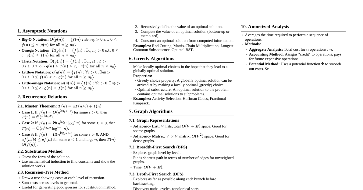
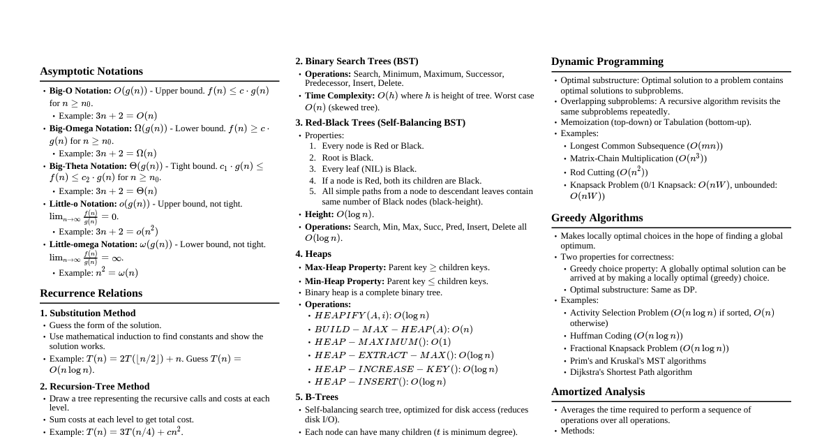
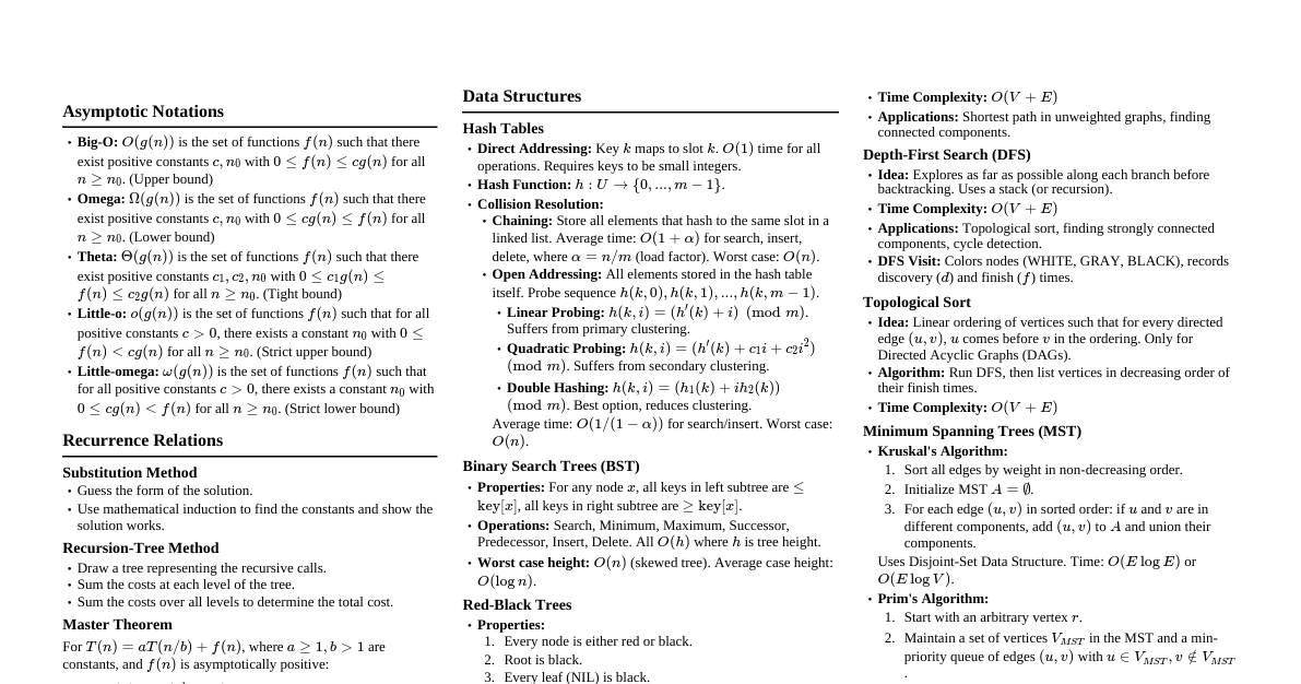
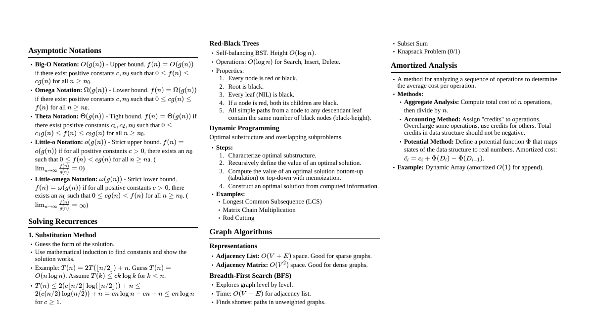
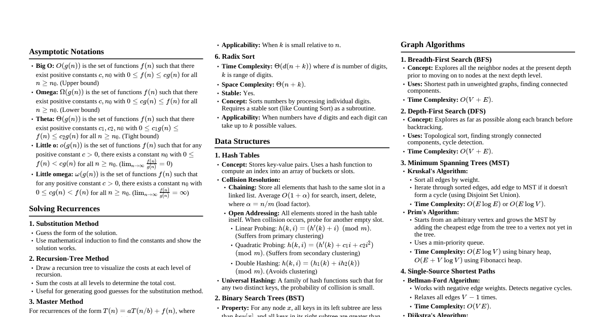
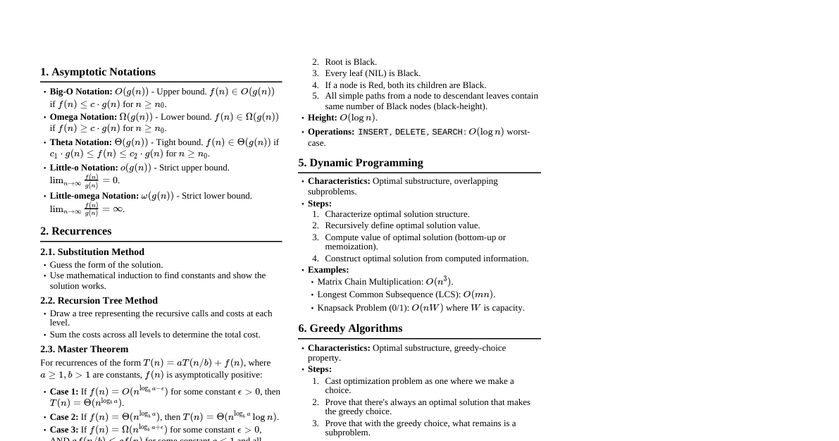
1. Asymptotic Notations Big-O Notation ($O$): Upper bound. $f(n) \in O(g(n))$ if $\exists c, n_0 > 0$ s.t. $0 \le f(n) \le c \cdot g(n)$ for all $n \ge n_0$. Omega Notation ($\Omega$): Lower bound. $f(n) \in \Omega(g(n))$ if $\exists c, n_0 > 0$ s.t. $0 \le c \cdot g(n) \le f(n)$ for all $n \ge n_0$. Theta Notation ($\Theta$): Tight bound. $f(n) \in \Theta(g(n))$ if $\exists c_1, c_2, n_0 > 0$ s.t. $0 \le c_1 \cdot g(n) \le f(n) \le c_2 \cdot g(n)$ for all $n \ge n_0$. Little-o Notation ($o$): Strict upper bound. $f(n) \in o(g(n))$ if $\lim_{n \to \infty} \frac{f(n)}{g(n)} = 0$. Little-omega Notation ($\omega$): Strict lower bound. $f(n) \in \omega(g(n))$ if $\lim_{n \to \infty} \frac{f(n)}{g(n)} = \infty$. 2. Sorting Algorithms 2.1. Comparison Sorts Algorithm Worst-case Time Average-case Time Best-case Time Space Stable Insertion Sort $O(n^2)$ $O(n^2)$ $O(n)$ $O(1)$ Yes Merge Sort $O(n \log n)$ $O(n \log n)$ $O(n \log n)$ $O(n)$ Yes Heap Sort $O(n \log n)$ $O(n \log n)$ $O(n \log n)$ $O(1)$ No Quick Sort $O(n^2)$ $O(n \log n)$ $O(n \log n)$ $O(\log n)$ No 2.2. Non-Comparison Sorts Counting Sort: $O(n+k)$ time, $O(n+k)$ space. $k$ is range of input integers. Stable. Radix Sort: $O(d(n+k))$ time, $O(n+k)$ space. $d$ is number of digits, $k$ is base. Stable. Bucket Sort: $O(n)$ average time, $O(n^2)$ worst-case. Assumes uniformly distributed input. 3. Recurrence Relations 3.1. Substitution Method Guess the form of the solution. Use mathematical induction to find constants and show it works. 3.2. Recursion-Tree Method Draw a recursion tree for the recurrence. Sum the costs at each level of the tree. Sum the costs of all levels to determine total cost. 3.3. Master Theorem For recurrences of the form $T(n) = aT(n/b) + f(n)$, where $a \ge 1, b > 1$ are constants, $f(n)$ is asymptotically positive: Case 1: If $f(n) = O(n^{\log_b a - \epsilon})$ for some constant $\epsilon > 0$, then $T(n) = \Theta(n^{\log_b a})$. Case 2: If $f(n) = \Theta(n^{\log_b a})$, then $T(n) = \Theta(n^{\log_b a} \log n)$. Case 3: If $f(n) = \Omega(n^{\log_b a + \epsilon})$ for some constant $\epsilon > 0$, AND $af(n/b) \le c f(n)$ for some constant $c 4. Data Structures 4.1. Hash Tables Direct Addressing: $O(1)$ time for all ops, but requires small key range. Chaining: Linked lists for collisions. Avg $O(1)$ if load factor $\alpha = n/m$ is $O(1)$. Worst $O(n)$. Open Addressing: Probing for empty slots. Linear Probing: $h(k, i) = (h'(k) + i) \pmod m$. Suffers from primary clustering. Quadratic Probing: $h(k, i) = (h'(k) + c_1 i + c_2 i^2) \pmod m$. Suffers from secondary clustering. Double Hashing: $h(k, i) = (h_1(k) + i \cdot h_2(k)) \pmod m$. Best collision resolution. 4.2. Binary Search Trees (BST) Properties: Left subtree keys root key. Operations: Search, Minimum, Maximum, Successor, Predecessor, Insert, Delete. All $O(h)$ where $h$ is height. Worst-case height $O(n)$ (skewed tree), best-case height $O(\log n)$ (balanced tree). 4.3. Red-Black Trees Self-balancing BST. Guarantees $O(\log n)$ height. Properties: Every node is Red or Black. Root is Black. Every leaf (NIL) is Black. If a node is Red, both its children are Black. All paths from a node to descendant leaves contain same number of Black nodes (Black-height). Insert/Delete: $O(\log n)$ time, involves rotations and color changes. 4.4. Heaps (Binary Heaps) Max-Heap: Parent key $\ge$ children keys. Min-Heap: Parent key $\le$ children keys. Operations: MAX-HEAPIFY(A, i) : $O(\log n)$. Maintains max-heap property. BUILD-MAX-HEAP(A) : $O(n)$. Builds max-heap from unsorted array. HEAPSORT(A) : $O(n \log n)$. Sorts in-place. HEAP-MAXIMUM() : $O(1)$. HEAP-EXTRACT-MAX() : $O(\log n)$. HEAP-INCREASE-KEY() : $O(\log n)$. MAX-HEAP-INSERT() : $O(\log n)$. 5. Dynamic Programming Optimal substructure: Optimal solution to a problem contains optimal solutions to subproblems. Overlapping subproblems: A recursive algorithm revisits the same subproblems repeatedly. Steps: Characterize optimal substructure. Recursively define the value of an optimal solution. Compute the value of an optimal solution (usually bottom-up). Construct an optimal solution from computed information (optional). Examples: Rod Cutting, Matrix-Chain Multiplication, Longest Common Subsequence, Optimal BST. 6. Greedy Algorithms Optimal substructure. Greedy-choice property: A globally optimal solution can be achieved by making a locally optimal (greedy) choice. Does not always yield optimal solution, but does for some problems. Examples: Activity Selection, Huffman Codes, Minimum Spanning Trees (Prim's, Kruskal's). 7. Graph Algorithms 7.1. Graph Representations Adjacency List: $O(V+E)$ space. Good for sparse graphs. Adjacency Matrix: $O(V^2)$ space. Good for dense graphs. 7.2. Breadth-First Search (BFS) Explores layer by layer. Finds shortest path in unweighted graphs. Time: $O(V+E)$. Uses a queue. 7.3. Depth-First Search (DFS) Explores as far as possible along each branch before backtracking. Time: $O(V+E)$. Uses a stack (or recursion). Used for topological sort, strongly connected components. 7.4. Minimum Spanning Trees (MST) Prim's Algorithm: Grows an MST from a starting vertex. $O(E \log V)$ with Fibonacci heap, $O(E \log V)$ with binary heap. Kruskal's Algorithm: Adds edges in increasing order of weight, avoiding cycles. $O(E \log E)$ or $O(E \log V)$ with disjoint-set data structure. 7.5. Shortest Paths Bellman-Ford: Single-source shortest paths in graphs with negative edge weights. Detects negative cycles. $O(VE)$ time. Dijkstra's Algorithm: Single-source shortest paths in graphs with non-negative edge weights. $O(E \log V)$ with binary heap. Floyd-Warshall: All-pairs shortest paths. $O(V^3)$ time. Can handle negative edges (no negative cycles). 8. Maximum Flow Flow Network: Directed graph $G=(V, E)$ with capacity $c(u,v) \ge 0$ for each edge $(u,v) \in E$. Source $s$, sink $t$. Flow $f$: A function $f: V \times V \to \mathbb{R}$ satisfying: Capacity constraint: $f(u,v) \le c(u,v)$. Skew symmetry: $f(u,v) = -f(v,u)$. Flow conservation: For all $u \in V - \{s,t\}$, $\sum_{v \in V} f(u,v) = 0$. Value of flow: $|f| = \sum_{v \in V} f(s,v)$. Ford-Fulkerson Method: Repeatedly finds augmenting paths in residual graph using BFS (Edmonds-Karp) or DFS. Edmonds-Karp: $O(VE^2)$ time. Max-Flow Min-Cut Theorem: The value of a maximum flow is equal to the capacity of a minimum cut. 9. NP-Completeness P: Class of problems solvable in polynomial time. NP: Class of problems verifiable in polynomial time (solution can be checked in poly time). NP-Hard: A problem $H$ is NP-hard if every problem in NP can be polynomial-time reduced to $H$. NP-Complete (NPC): A problem $C$ is NP-complete if $C \in \text{NP}$ and $C$ is NP-hard. Reduction: $L_1 \le_P L_2$ means problem $L_1$ can be transformed into $L_2$ in polynomial time. If $L_1 \le_P L_2$ and $L_1$ is NP-hard, then $L_2$ is NP-hard. Examples of NPC Problems: SAT, 3-SAT, Clique, Vertex Cover, Hamiltonian Cycle, Traveling Salesperson Problem, Subset Sum.