Introduction to Algorithms (CLRS)

Cheatsheet Content

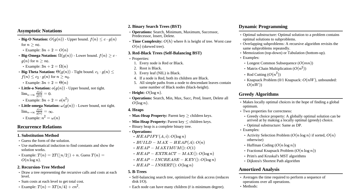
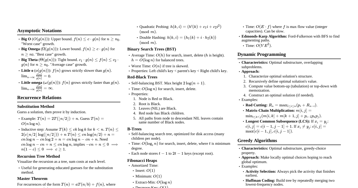
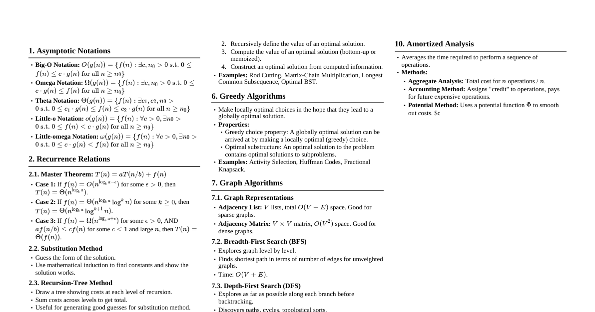
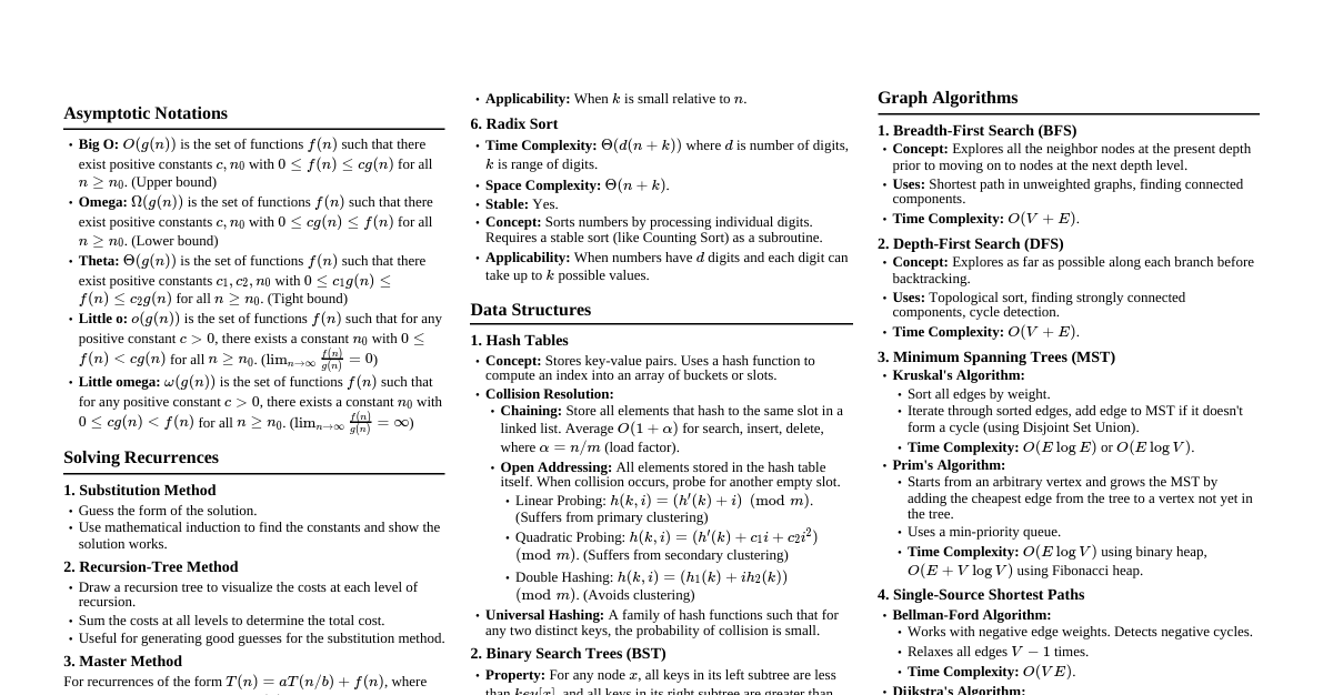
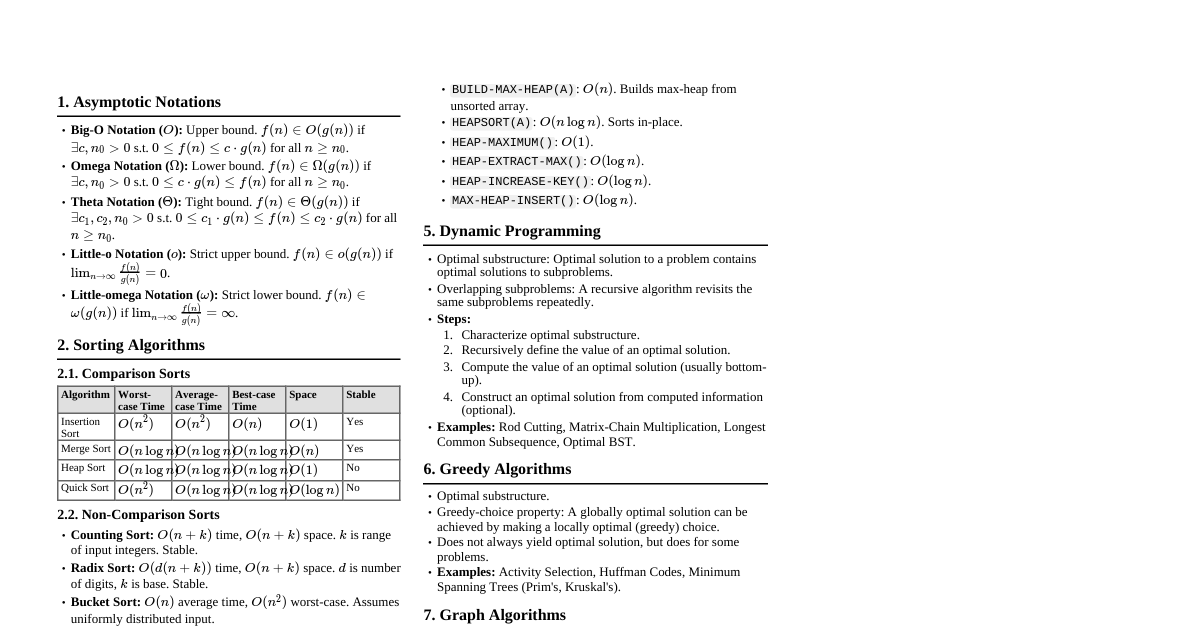
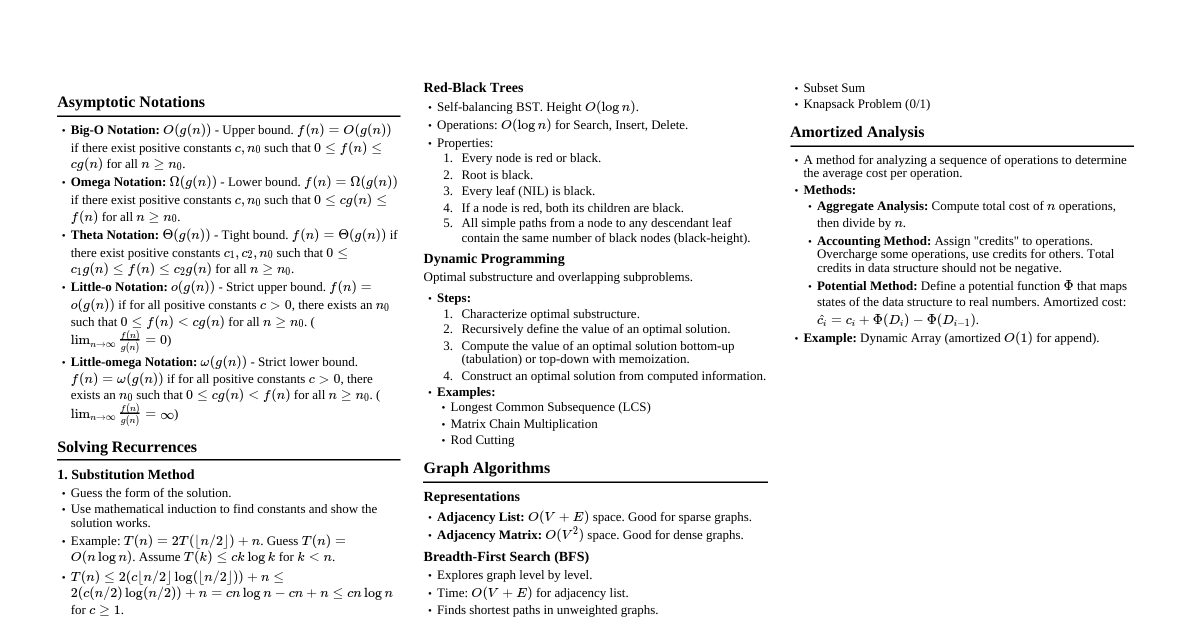
Asymptotic Notations Big-O: $O(g(n))$ is the set of functions $f(n)$ such that there exist positive constants $c, n_0$ with $0 \le f(n) \le c g(n)$ for all $n \ge n_0$. (Upper bound) Omega: $\Omega(g(n))$ is the set of functions $f(n)$ such that there exist positive constants $c, n_0$ with $0 \le c g(n) \le f(n)$ for all $n \ge n_0$. (Lower bound) Theta: $\Theta(g(n))$ is the set of functions $f(n)$ such that there exist positive constants $c_1, c_2, n_0$ with $0 \le c_1 g(n) \le f(n) \le c_2 g(n)$ for all $n \ge n_0$. (Tight bound) Little-o: $o(g(n))$ is the set of functions $f(n)$ such that for all positive constants $c > 0$, there exists a constant $n_0$ with $0 \le f(n) Little-omega: $\omega(g(n))$ is the set of functions $f(n)$ such that for all positive constants $c > 0$, there exists a constant $n_0$ with $0 \le c g(n) Recurrence Relations Substitution Method Guess the form of the solution. Use mathematical induction to find the constants and show the solution works. Recursion-Tree Method Draw a tree representing the recursive calls. Sum the costs at each level of the tree. Sum the costs over all levels to determine the total cost. Master Theorem For $T(n) = aT(n/b) + f(n)$, where $a \ge 1, b > 1$ are constants, and $f(n)$ is asymptotically positive: If $f(n) = O(n^{\log_b a - \epsilon})$ for some constant $\epsilon > 0$, then $T(n) = \Theta(n^{\log_b a})$. If $f(n) = \Theta(n^{\log_b a})$, then $T(n) = \Theta(n^{\log_b a} \log n)$. If $f(n) = \Omega(n^{\log_b a + \epsilon})$ for some constant $\epsilon > 0$, AND if $a f(n/b) \le c f(n)$ for some constant $c Sorting Algorithms Insertion Sort Idea: Build the final sorted array one item at a time. Takes elements from the input data and inserts them into the correct position in the sorted array. Time Complexity: Best: $\Theta(n)$, Average: $\Theta(n^2)$, Worst: $\Theta(n^2)$ Space Complexity: $O(1)$ Stable: Yes Merge Sort Idea: Divide and conquer. Divides array into two halves, recursively sorts them, then merges the two sorted halves. Time Complexity: All cases: $\Theta(n \log n)$ Space Complexity: $O(n)$ (for temporary array in merge) Stable: Yes Heap Sort Idea: Uses a binary heap data structure. Builds a max-heap from input data, then repeatedly extracts the maximum element and rebuilds the heap. Time Complexity: All cases: $\Theta(n \log n)$ Space Complexity: $O(1)$ (in-place) Stable: No Quick Sort Idea: Divide and conquer. Picks an element as a pivot and partitions the array around the pivot. Time Complexity: Best: $\Theta(n \log n)$, Average: $\Theta(n \log n)$, Worst: $\Theta(n^2)$ Space Complexity: $O(\log n)$ (average, due to recursion stack), $O(n)$ (worst) Stable: No Counting Sort Idea: Non-comparative integer sorting algorithm. Counts the number of occurrences of each distinct element and uses arithmetic to determine the positions of each element in the output sequence. Time Complexity: $\Theta(n+k)$ where $k$ is the range of input numbers. Space Complexity: $\Theta(n+k)$ Stable: Yes Constraint: Works best when $k$ is not significantly larger than $n$. Radix Sort Idea: Non-comparative integer sorting algorithm. Sorts numbers by processing individual digits. Typically uses counting sort as a subroutine. Time Complexity: $\Theta(d(n+k))$ where $d$ is the number of digits, $k$ is the range of digits. Space Complexity: $\Theta(n+k)$ Stable: Yes Data Structures Hash Tables Direct Addressing: Key $k$ maps to slot $k$. $O(1)$ time for all operations. Requires keys to be small integers. Hash Function: $h: U \to \{0, ..., m-1\}$. Collision Resolution: Chaining: Store all elements that hash to the same slot in a linked list. Average time: $O(1+\alpha)$ for search, insert, delete, where $\alpha = n/m$ (load factor). Worst case: $O(n)$. Open Addressing: All elements stored in the hash table itself. Probe sequence $h(k, 0), h(k, 1), ..., h(k, m-1)$. Linear Probing: $h(k, i) = (h'(k) + i) \pmod m$. Suffers from primary clustering. Quadratic Probing: $h(k, i) = (h'(k) + c_1 i + c_2 i^2) \pmod m$. Suffers from secondary clustering. Double Hashing: $h(k, i) = (h_1(k) + i h_2(k)) \pmod m$. Best option, reduces clustering. Average time: $O(1/(1-\alpha))$ for search/insert. Worst case: $O(n)$. Binary Search Trees (BST) Properties: For any node $x$, all keys in left subtree are $\le \text{key}[x]$, all keys in right subtree are $\ge \text{key}[x]$. Operations: Search, Minimum, Maximum, Successor, Predecessor, Insert, Delete. All $O(h)$ where $h$ is tree height. Worst case height: $O(n)$ (skewed tree). Average case height: $O(\log n)$. Red-Black Trees Properties: Every node is either red or black. Root is black. Every leaf (NIL) is black. If a node is red, both its children are black. All simple paths from a node to any descendant leaf contain the same number of black nodes (black-height). Height: Max height is $2 \log_2(n+1)$. All operations $O(\log n)$. Rotations: Left-Rotate, Right-Rotate maintain BST property and help balance. B-Trees Properties (degree $t \ge 2$): Every node has at most $2t-1$ keys and $2t$ children. Every node (except root) has at least $t-1$ keys and $t$ children. Root has at least 1 key (if not a leaf). All leaves have the same depth. Height: $O(\log_t n)$. All operations (Search, Insert, Delete) $O(t \log_t n)$. Optimized for disk access (minimize disk I/Os). Dynamic Programming Characteristics: Optimal Substructure: Optimal solution to a problem contains optimal solutions to subproblems. Overlapping Subproblems: A recursive algorithm revisits the same subproblems repeatedly. Approach: Characterize the structure of an optimal solution. Recursively define the value of an optimal solution. Compute the value of an optimal solution (bottom-up or memoization). Construct an optimal solution from computed information. Examples: Rod Cutting: $R_n = \max_{1 \le i \le n} (p_i + R_{n-i})$. Matrix-Chain Multiplication: $m[i,j] = \min_{i \le k Longest Common Subsequence (LCS): If $x_i = y_j$: $c[i,j] = c[i-1,j-1] + 1$. If $x_i \ne y_j$: $c[i,j] = \max(c[i-1,j], c[i,j-1])$. Greedy Algorithms Characteristics: Optimal Substructure: (Same as DP) Greedy-choice property: A globally optimal solution can be arrived at by making a locally optimal (greedy) choice. Approach: Make the choice that seems best at the current moment, then solve the remaining subproblem. Examples: Activity Selection: Always choose the activity that finishes earliest among those compatible with previously selected activities. Huffman Codes: Build a binary tree where lowest frequency characters are merged first. Kruskal's Algorithm: Add the cheapest edge that connects two previously disconnected components. Prim's Algorithm: Grow a single tree from a starting vertex, always adding the cheapest edge connecting a vertex in the tree to one outside. Graph Algorithms Breadth-First Search (BFS) Idea: Explores all nodes at the present depth level before moving on to nodes at the next depth level. Uses a queue. Time Complexity: $O(V+E)$ Applications: Shortest path in unweighted graphs, finding connected components. Depth-First Search (DFS) Idea: Explores as far as possible along each branch before backtracking. Uses a stack (or recursion). Time Complexity: $O(V+E)$ Applications: Topological sort, finding strongly connected components, cycle detection. DFS Visit: Colors nodes (WHITE, GRAY, BLACK), records discovery ($d$) and finish ($f$) times. Topological Sort Idea: Linear ordering of vertices such that for every directed edge $(u,v)$, $u$ comes before $v$ in the ordering. Only for Directed Acyclic Graphs (DAGs). Algorithm: Run DFS, then list vertices in decreasing order of their finish times. Time Complexity: $O(V+E)$ Minimum Spanning Trees (MST) Kruskal's Algorithm: Sort all edges by weight in non-decreasing order. Initialize MST $A = \emptyset$. For each edge $(u,v)$ in sorted order: if $u$ and $v$ are in different components, add $(u,v)$ to $A$ and union their components. Uses Disjoint-Set Data Structure. Time: $O(E \log E)$ or $O(E \log V)$. Prim's Algorithm: Start with an arbitrary vertex $r$. Maintain a set of vertices $V_{MST}$ in the MST and a min-priority queue of edges $(u,v)$ with $u \in V_{MST}, v \notin V_{MST}$. Repeatedly extract minimum-weight edge from priority queue, add $v$ to $V_{MST}$, and update neighbors' keys. Time: $O(E \log V)$ with binary heap, $O(E + V \log V)$ with Fibonacci heap. Shortest Paths Single-Source Shortest Paths (SSSP): Bellman-Ford: Handles negative edge weights. Detects negative cycles. Time: $O(VE)$. Dijkstra's Algorithm: For non-negative edge weights. Uses a min-priority queue. Time: $O(E \log V)$ with binary heap, $O(E + V \log V)$ with Fibonacci heap. All-Pairs Shortest Paths (APSP): Floyd-Warshall: Dynamic programming. Allows negative edge weights. Time: $O(V^3)$. Johnson's Algorithm: Reweights graph to use Dijkstra's. Handles negative edge weights (but no negative cycles). Time: $O(VE + V^2 \log V)$. Maximum Flow Flow Network: Directed graph $G=(V,E)$ with capacities $c(u,v) \ge 0$. Flow: $f(u,v)$ satisfying capacity, skew symmetry, and flow conservation. Residual Graph: $G_f$ with residual capacities $c_f(u,v)$. Augmenting Path: A path from source $s$ to sink $t$ in $G_f$. Ford-Fulkerson Method: Repeatedly find augmenting paths and push flow along them until no more paths exist. Edmonds-Karp: Uses BFS to find augmenting paths. Time: $O(VE^2)$. Max-Flow Min-Cut Theorem: The value of a maximum $s-t$ flow is equal to the capacity of a minimum $s-t$ cut. Complexity Classes P: Class of problems solvable in polynomial time by a deterministic Turing machine. NP: Class of problems whose solutions can be verified in polynomial time by a deterministic Turing machine (or solvable in polynomial time by a non-deterministic Turing machine). NP-Hard: A problem $H$ is NP-hard if for every problem $L$ in NP, $L$ is polynomial-time reducible to $H$ ($L \le_p H$). NP-Complete: A problem $C$ is NP-complete if $C \in \text{NP}$ and $C$ is NP-hard. Examples of NP-Complete Problems: Satisfiability (SAT), Traveling Salesperson Problem (TSP), Clique, Vertex Cover, Hamiltonian Cycle.