LSTM & GRU Cheatsheet

Cheatsheet Content

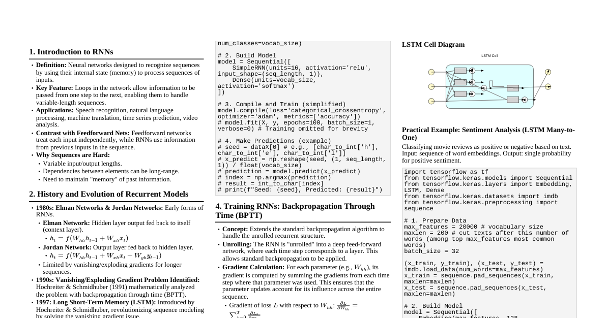
Recurrent Neural Networks (RNNs) Limitations The state ($s_t$) of an RNN records information from all previous time steps. At each new timestep, old information gets morphed by the current input. Information from earlier time steps ($t-k$) gets completely morphed, making it impossible to extract original information by time $t$. Similar problems occur with information flow backwards (backpropagation), making it hard to assign error responsibility to past events (vanishing gradients). Whiteboard Analogy for Selective Memory Imagine the RNN state as a fixed-size whiteboard. At each time step, we: Selectively write: Choose what new information to add to the board. Selectively read: Decide which existing information to use for current decisions. Selectively forget (erase): Remove obsolete or less useful information when the board is full. This analogy highlights the need for RNNs to manage their finite state effectively to retain important long-term dependencies. Sentiment Prediction Example Task: Predict sentiment (positive/negative) of a review. RNN reads the document word by word, updating its state. Problem: Information from early words can be lost by the end of a long document. Ideal Behavior: Forget: Information from stop words (a, the, etc.). Selectively Read: Information from previous sentiment-bearing words (awesome, amazing). Selectively Write: New information from the current word to the state. The blue vector ($s_t$) in RNNs is the state, having finite size ($s_t \in \mathbb{R}^n$). It can get overloaded, causing early information to be lost. LSTM and GRU aim to address this. Long Short-Term Memory (LSTM) LSTMs use "gates" to control the flow of information into and out of the cell state, allowing them to selectively remember or forget information. 1. Output Gate ($o_t$) - Selective Write Decides what fraction of the current cell state ($c_t$) to pass on to the hidden state ($h_t$). Computed as: $o_t = \sigma(W_o h_{t-1} + U_o x_t + b_o)$ $h_t = o_t \odot \tanh(c_t)$ The sigmoid function $\sigma$ restricts values between 0 and 1, acting as a "gate." 2. Input Gate ($i_t$) - Selective Read Decides which new information from the current input ($x_t$) and previous hidden state ($h_{t-1}$) to store in the cell state. Computed as: $i_t = \sigma(W_i h_{t-1} + U_i x_t + b_i)$ A candidate cell state $\tilde{c}_t$ is also computed: $\tilde{c}_t = \tanh(W_c h_{t-1} + U_c x_t + b_c)$ 3. Forget Gate ($f_t$) - Selective Forget Decides which information to discard from the previous cell state ($c_{t-1}$). Computed as: $f_t = \sigma(W_f h_{t-1} + U_f x_t + b_f)$ 4. Cell State Update ($c_t$) The core memory of the LSTM, updated based on the forget gate, input gate, and candidate cell state. $c_t = f_t \odot c_{t-1} + i_t \odot \tilde{c}_t$ The updated cell state $c_t$ then influences the next hidden state $h_t$. Summary of LSTM Equations: Forget Gate: $f_t = \sigma(W_f h_{t-1} + U_f x_t + b_f)$ Input Gate: $i_t = \sigma(W_i h_{t-1} + U_i x_t + b_i)$ Candidate Cell State: $\tilde{c}_t = \tanh(W_c h_{t-1} + U_c x_t + b_c)$ Cell State: $c_t = f_t \odot c_{t-1} + i_t \odot \tilde{c}_t$ Output Gate: $o_t = \sigma(W_o h_{t-1} + U_o x_t + b_o)$ Hidden State: $h_t = o_t \odot \tanh(c_t)$ Gated Recurrent Units (GRUs) GRUs are a simpler variant of LSTMs, combining the forget and input gates into a single "update" gate, and merging the cell state and hidden state. 1. Update Gate ($z_t$) Combines the functionality of LSTM's forget and input gates. It decides how much of the past information to keep and how much new information to add. Computed as: $z_t = \sigma(W_z h_{t-1} + U_z x_t + b_z)$ 2. Reset Gate ($r_t$) Determines how much of the previous hidden state ($h_{t-1}$) to "forget" when computing the new candidate hidden state. Computed as: $r_t = \sigma(W_r h_{t-1} + U_r x_t + b_r)$ 3. Candidate Hidden State ($\tilde{h}_t$) This is a new hidden state that might be proposed, similar to LSTM's candidate cell state. The reset gate influences how much of the previous hidden state is considered. Computed as: $\tilde{h}_t = \tanh(W(r_t \odot h_{t-1}) + U x_t + b)$ 4. Hidden State Update ($h_t$) The final hidden state is a linear interpolation between the previous hidden state and the candidate hidden state, controlled by the update gate. Computed as: $h_t = (1 - z_t) \odot h_{t-1} + z_t \odot \tilde{h}_t$ Summary of GRU Equations: Update Gate: $z_t = \sigma(W_z h_{t-1} + U_z x_t + b_z)$ Reset Gate: $r_t = \sigma(W_r h_{t-1} + U_r x_t + b_r)$ Candidate Hidden State: $\tilde{h}_t = \tanh(W(r_t \odot h_{t-1}) + U x_t + b)$ Hidden State: $h_t = (1 - z_t) \odot h_{t-1} + z_t \odot \tilde{h}_t$