Recurrent Neural Networks
Cheatsheet Content
1. Introduction to RNNs Definition: Neural networks designed to recognize sequences by using their internal state (memory) to process sequences of inputs. Key Feature: Loops in the network allow information to be passed from one step to the next, enabling them to handle variable-length sequences. Applications: Speech recognition, natural language processing, machine translation, time series prediction, video analysis. Contrast with Feedforward Nets: Feedforward networks treat each input independently, while RNNs use information from previous inputs in the sequence. Why Sequences are Hard: Variable input/output lengths. Dependencies between elements can be long-range. Need to maintain "memory" of past information. 2. History and Evolution of Recurrent Models 1980s: Elman Networks & Jordan Networks: Early forms of RNNs. Elman Network: Hidden layer output fed back to itself (context layer). $h_t = f(W_{hh} h_{t-1} + W_{xh} x_t)$ Jordan Network: Output layer fed back to hidden layer. $h_t = f(W_{hh} h_{t-1} + W_{xh} x_t + W_{yh} y_{t-1})$ Limited by vanishing/exploding gradients for longer sequences. 1990s: Vanishing/Exploding Gradient Problem Identified: Hochreiter & Schmidhuber (1991) mathematically analyzed the problem with backpropagation through time (BPTT). 1997: Long Short-Term Memory (LSTM): Introduced by Hochreiter & Schmidhuber, revolutionizing sequence modeling by solving the vanishing gradient issue. 2014: Gated Recurrent Unit (GRU): Introduced by Cho et al., a simpler variant of LSTM with comparable performance. 2015-2017: Attention Mechanisms: Introduced by Bahdanau et al. (2015) and Luong et al. (2015) to improve Seq2Seq models, allowing decoders to 'look back' at relevant encoder states. 2017: Transformers: Introduced by Vaswani et al. ("Attention Is All You Need"), completely replacing recurrence with self-attention, enabling parallelization and state-of-the-art performance in many NLP tasks. 3. Basic RNN Structure and Equations Input Sequence: $x = (x_1, x_2, ..., x_T)$, where $x_t \in \mathbb{R}^{D_x}$ (input dimension). Hidden State Sequence: $h = (h_1, h_2, ..., h_T)$, where $h_t \in \mathbb{R}^{D_h}$ (hidden state dimension). Output Sequence: $y = (y_1, y_2, ..., y_T)$ (or a single $y_T$), where $y_t \in \mathbb{R}^{D_y}$ (output dimension). Recurrence Relation (Simple RNN Cell): $h_t = \tanh(W_{hh} h_{t-1} + W_{xh} x_t + b_h)$ $y_t = W_{hy} h_t + b_y$ (often followed by activation like softmax for classification) Where: $W_{hh} \in \mathbb{R}^{D_h \times D_h}$ (weights for previous hidden state) $W_{xh} \in \mathbb{R}^{D_h \times D_x}$ (weights for current input) $W_{hy} \in \mathbb{R}^{D_y \times D_h}$ (weights for current output) $b_h \in \mathbb{R}^{D_h}$, $b_y \in \mathbb{R}^{D_y}$ (biases) $h_0$ is usually initialized to a zero vector. RNN Unrolled Diagram RNN $x_{t-1}$ $y_{t-1}$ RNN $x_t$ $y_t$ RNN $x_{t+1}$ $y_{t+1}$ $h_{t-1}$ $h_t$ ... ... Practical Example: Character-level Language Model (Simple RNN) Predicting the next character in a sequence. Input: one-hot encoded characters. Output: probability distribution over next character. import numpy as np import tensorflow as tf from tensorflow.keras.models import Sequential from tensorflow.keras.layers import SimpleRNN, Dense, Embedding # 1. Prepare Data text = "hello world" chars = sorted(list(set(text))) char_to_int = dict((c, i) for i, c in enumerate(chars)) int_to_char = dict((i, c) for i, c in enumerate(chars)) vocab_size = len(chars) seq_length = 3 # e.g., predict 'l' from 'hel' dataX = [] dataY = [] for i in range(0, len(text) - seq_length, 1): seq_in = text[i:i + seq_length] seq_out = text[i + seq_length] dataX.append([char_to_int[char] for char in seq_in]) dataY.append(char_to_int[seq_out]) X = np.reshape(dataX, (len(dataX), seq_length, 1)) X = X / float(vocab_size) # Normalize input y = tf.keras.utils.to_categorical(dataY, num_classes=vocab_size) # 2. Build Model model = Sequential([ SimpleRNN(units=16, activation='relu', input_shape=(seq_length, 1)), Dense(units=vocab_size, activation='softmax') ]) # 3. Compile and Train (simplified) model.compile(loss='categorical_crossentropy', optimizer='adam', metrics=['accuracy']) # model.fit(X, y, epochs=100, batch_size=1, verbose=0) # Training omitted for brevity # 4. Make Predictions (example) # seed = dataX[0] # e.g., [char_to_int['h'], char_to_int['e'], char_to_int['l']] # x_predict = np.reshape(seed, (1, seq_length, 1)) / float(vocab_size) # prediction = model.predict(x_predict) # index = np.argmax(prediction) # result = int_to_char[index] # print(f"Seed: {seed}, Predicted: {result}") 4. Training RNNs: Backpropagation Through Time (BPTT) Concept: Extends the standard backpropagation algorithm to handle the unrolled recurrent structure. Unrolling: The RNN is "unrolled" into a deep feed-forward network, where each time step corresponds to a layer. This allows standard backpropagation to be applied. Gradient Calculation: For each parameter (e.g., $W_{hh}$), its gradient is computed by summing the gradients from each time step where that parameter was used. This ensures that the parameter updates account for its influence across the entire sequence. Gradient of loss $L$ with respect to $W_{hh}$: $\frac{\partial L}{\partial W_{hh}} = \sum_{k=0}^{T} \frac{\partial L_k}{\partial W_{hh}}$ Where $L_k$ is the loss at time step $k$. Challenges: Vanishing Gradients: Gradients can shrink exponentially as they propagate back through many time steps. This occurs because repeated multiplication by small values (e.g., from tanh derivatives) causes gradients to become negligible, making it difficult for the network to learn long-term dependencies. Exploding Gradients: Gradients can grow exponentially, leading to very large weight updates that destabilize the network and cause divergence. This often happens due to repeated multiplication by large values. Solutions: For Exploding Gradients: Gradient Clipping (rescaling gradients if their L2 norm exceeds a certain threshold). For Vanishing Gradients: More sophisticated RNN architectures like LSTMs and GRUs, which use gating mechanisms to control information flow. 5. Long Short-Term Memory (LSTM) Networks Purpose: Specifically designed to address the vanishing gradient problem and effectively capture long-term dependencies in sequences. Core Idea: Introduce a "cell state" ($C_t$) that runs through the entire sequence, acting as a conveyor belt for information. "Gates" (sigmoid-activated neural networks) regulate the flow of information into and out of this cell state. Components (Gates): Each gate outputs a value between 0 and 1, controlling how much information passes through. Forget Gate ($f_t$): Decides what information from the previous cell state ($C_{t-1}$) should be discarded. A 0 means "completely forget," a 1 means "completely keep." $f_t = \sigma(W_f \cdot [h_{t-1}, x_t] + b_f)$ Input Gate ($i_t$): Decides what new information from the current input ($x_t$) and previous hidden state ($h_{t-1}$) should be stored in the cell state. This involves two parts: $i_t = \sigma(W_i \cdot [h_{t-1}, x_t] + b_i)$ (decides which values to update) $\tilde{C}_t = \tanh(W_C \cdot [h_{t-1}, x_t] + b_C)$ (generates a vector of new candidate values) Update Cell State: The previous cell state $C_{t-1}$ is updated to $C_t$ by element-wise multiplication with the forget gate output (forgetting) and element-wise addition of the input gate output multiplied by the candidate values (adding new information). $C_t = f_t \odot C_{t-1} + i_t \odot \tilde{C}_t$ Output Gate ($o_t$): Decides what parts of the cell state ($C_t$) should be output as the new hidden state ($h_t$). The cell state is first passed through $\tanh$ to squish values between -1 and 1. $o_t = \sigma(W_o \cdot [h_{t-1}, x_t] + b_o)$ $h_t = o_t \odot \tanh(C_t)$ Activation Functions: The sigmoid function ($\sigma$) outputs values between 0 and 1 (for gates), while the hyperbolic tangent function ($\tanh$) outputs values between -1 and 1 (for candidate cell state and final hidden state). LSTM Cell Diagram LSTM Cell $x_t$ $h_{t-1}$ $C_{t-1}$ $h_t$ $C_t$ $\sigma_f$ x $\sigma_i$ x $\tanh_C$ x $\sigma_o$ x $\tanh_C$ + Practical Example: Sentiment Analysis (LSTM Many-to-One) Classifying movie reviews as positive or negative based on text. Input: sequence of word embeddings. Output: single probability for positive sentiment. import tensorflow as tf from tensorflow.keras.models import Sequential from tensorflow.keras.layers import Embedding, LSTM, Dense from tensorflow.keras.datasets import imdb from tensorflow.keras.preprocessing import sequence # 1. Prepare Data max_features = 20000 # vocabulary size maxlen = 200 # cut texts after this number of words (among top max_features most common words) batch_size = 32 (x_train, y_train), (x_test, y_test) = imdb.load_data(num_words=max_features) x_train = sequence.pad_sequences(x_train, maxlen=maxlen) x_test = sequence.pad_sequences(x_test, maxlen=maxlen) # 2. Build Model model = Sequential([ Embedding(max_features, 128, input_length=maxlen), # Turns positive integers (indexes) into dense vectors of fixed size LSTM(units=128), # Returns a single vector (many-to-one) Dense(units=1, activation='sigmoid') # Binary classification ]) # 3. Compile and Train (simplified) model.compile(optimizer='adam', loss='binary_crossentropy', metrics=['accuracy']) # model.fit(x_train, y_train, epochs=10, batch_size=batch_size, validation_data=(x_test, y_test)) model.summary() 6. Gated Recurrent Unit (GRU) Networks Purpose: A simplified yet powerful alternative to LSTMs, also effective at handling long-term dependencies and mitigating vanishing gradients. Fewer Gates: GRUs combine the forget and input gates into a single "update gate" and merge the cell state and hidden state, leading to a less complex structure with fewer parameters. Components: Update Gate ($z_t$): Controls how much of the previous hidden state ($h_{t-1}$) should be carried over to the current hidden state ($h_t$), and how much of the new candidate hidden state ($\tilde{h}_t$) should be used. $z_t = \sigma(W_z \cdot [h_{t-1}, x_t] + b_z)$ Reset Gate ($r_t$): Determines how much of the previous hidden state ($h_{t-1}$) to "forget" when calculating the new candidate hidden state ($\tilde{h}_t$). A small $r_t$ means $h_{t-1}$ is mostly ignored. $r_t = \sigma(W_r \cdot [h_{t-1}, x_t] + b_r)$ Candidate Hidden State ($\tilde{h}_t$): The potential new hidden state, calculated based on the current input and a "reset" version of the previous hidden state. $\tilde{h}_t = \tanh(W_h \cdot [r_t \odot h_{t-1}, x_t] + b_h)$ Hidden State Update: The final hidden state $h_t$ is a linear interpolation between the previous hidden state $h_{t-1}$ and the candidate hidden state $\tilde{h}_t$, controlled by the update gate $z_t$. $h_t = (1 - z_t) \odot h_{t-1} + z_t \odot \tilde{h}_t$ Advantages: Often faster to train and requires less data due to fewer parameters compared to LSTMs. Performance is frequently comparable, making GRUs a popular choice for many tasks. Practical Example: Time Series Forecasting (GRU Many-to-One) Predicting the next value in a sequence (e.g., stock price, temperature). Input: window of past values. Output: single future value. import numpy as np import tensorflow as tf from tensorflow.keras.models import Sequential from tensorflow.keras.layers import GRU, Dense # 1. Prepare Data (simplified sinusoidal wave) time_steps = np.linspace(0, 100, 1000) data = np.sin(time_steps / 10) + np.random.normal(0, 0.1, 1000) data = data.reshape(-1, 1) # (timesteps, features) # Create sequences for training def create_sequences(data, seq_length): X, y = [], [] for i in range(len(data) - seq_length): X.append(data[i:(i + seq_length)]) y.append(data[i + seq_length]) return np.array(X), np.array(y) seq_length = 10 X, y = create_sequences(data, seq_length) # Split into train/test (simplified) train_size = int(len(X) * 0.8) X_train, y_train = X[:train_size], y[:train_size] X_test, y_test = X[train_size:], y[train_size:] # 2. Build Model model = Sequential([ GRU(units=50, activation='tanh', input_shape=(seq_length, 1)), Dense(units=1) # Predict a single future value ]) # 3. Compile and Train (simplified) model.compile(optimizer='adam', loss='mse') # model.fit(X_train, y_train, epochs=20, batch_size=32, validation_data=(X_test, y_test)) model.summary() 7. Bidirectional RNNs (BiRNNs) Concept: Enhance RNNs by allowing them to process the input sequence in both forward and backward directions independently. This provides the model with context from both the past and the future for each point in the sequence. Architecture: Consists of two separate hidden layers: A forward layer processes the sequence from left-to-right (e.g., $x_1 \to x_2 \to ... \to x_T$), producing hidden states $\vec{h}_t$. A backward layer processes the sequence from right-to-left (e.g., $x_T \to x_{T-1} \to ... \to x_1$), producing hidden states $\overleftarrow{h}_t$. Combined Output: The final output at time $t$ is typically based on the concatenation or summation of both hidden states: $h_t = [\vec{h}_t; \overleftarrow{h}_t]$ (concatenation is common). This combined representation is then passed to the output layer. Benefit: Allows the network to utilize context from both past and future time steps, which is crucial for tasks where understanding the full context of a word or event is necessary (e.g., "apple" as a company vs. a fruit). Useful for tasks like speech recognition, machine translation, and named entity recognition. Limitation: Cannot be used for real-time prediction tasks where the entire future sequence is not yet available (e.g., predicting the next word in a live conversation). Practical Example: Named Entity Recognition (BiLSTM Many-to-Many) Identifying and classifying named entities (e.g., person, organization, location) in text. Input: sequence of word embeddings. Output: sequence of tags (one tag per word). import tensorflow as tf from tensorflow.keras.models import Sequential from tensorflow.keras.layers import Embedding, Bidirectional, LSTM, Dense, TimeDistributed from tensorflow.keras.preprocessing.sequence import pad_sequences import numpy as np # 1. Prepare Data (simplified example) # Assume you have word_to_idx, tag_to_idx, and padded sequences X, y # X_data: [[word_idx1, word_idx2, ...], ...] # y_data: [[tag_idx1, tag_idx2, ...], ...] vocab_size = 10000 # Example vocabulary size embedding_dim = 100 max_len = 50 # Max sequence length num_tags = 5 # e.g., O, B-PER, I-PER, B-LOC, I-LOC # Dummy data for demonstration X_train = np.random.randint(0, vocab_size, size=(100, max_len)) y_train = np.random.randint(0, num_tags, size=(100, max_len)) y_train = tf.keras.utils.to_categorical(y_train, num_classes=num_tags) # One-hot encode tags # 2. Build Model model = Sequential([ Embedding(vocab_size, embedding_dim, input_length=max_len), Bidirectional(LSTM(units=128, return_sequences=True)), # return_sequences=True for sequence output TimeDistributed(Dense(units=num_tags, activation='softmax')) # Apply Dense to each timestep ]) # 3. Compile and Train (simplified) model.compile(optimizer='adam', loss='categorical_crossentropy', metrics=['accuracy']) # model.fit(X_train, y_train, epochs=5, batch_size=32) model.summary() 8. Encoder-Decoder Architectures (Seq2Seq Models) Purpose: Designed for tasks that involve transforming an input sequence into an output sequence of potentially different length and content. Crucial for machine translation, text summarization, and chatbots. Components: Encoder: An RNN (often LSTM or GRU) that reads the entire input sequence (e.g., source language sentence) and compresses all its information into a fixed-size "context vector" (also known as a "thought vector" or "summary vector"). The final hidden and cell states of the encoder are typically used as this context. Decoder: Another RNN that takes the context vector as its initial hidden state and generates the output sequence (e.g., target language sentence) one element at a time. Each output depends on the context vector, its own previous hidden state, and the previously generated output token. Mechanism: Encoder: $C = \text{Encoder}(x_1, ..., x_T)$ (where $C$ is usually the final $h_T$ and $C_T$ of the encoder). Decoder: At each step $t$, the decoder takes the previous output $y_{t-1}$ (or a special START token for the first step), its previous hidden state $h_{t-1}$, and the context vector $C$ to produce the current hidden state $h_t$ and output $y_t$. $h_t = \text{DecoderCell}(h_{t-1}, y_{t-1}, C)$ $y_t = \text{OutputLayer}(h_t)$ Limitation: The fixed-size context vector can become a bottleneck for very long input sequences. It struggles to encapsulate all necessary information, leading to performance degradation for long sentences. This is where attention mechanisms become vital. Encoder-Decoder Diagram Encoder RNN RNN RNN $x_1$ $x_2$ $x_T$ C Decoder RNN RNN $y_1$ $y_M$ $y_1$ ... ... Practical Example: Machine Translation (Seq2Seq with Keras) Translating sentences from source to target language. This is a simplified version without attention. import numpy as np import tensorflow as tf from tensorflow.keras.models import Model from tensorflow.keras.layers import Input, LSTM, Dense from tensorflow.keras.preprocessing.text import Tokenizer from tensorflow.keras.preprocessing.sequence import pad_sequences # 1. Prepare Data (highly simplified for illustration) input_texts = ["go .", "hi .", "run .", "wow .", "run fast ."] target_texts = ["va !", "salut !", "cours !", "wow !", "cours vite !"] target_texts_input = [" va !", " salut !", " cours !", " wow !", " cours vite !"] # Tokenize input and target texts input_tokenizer = Tokenizer(filters='') input_tokenizer.fit_on_texts(input_texts) input_sequences = input_tokenizer.texts_to_sequences(input_texts) word_to_idx_input = input_tokenizer.word_index num_encoder_tokens = len(word_to_idx_input) + 1 target_tokenizer = Tokenizer(filters='') target_tokenizer.fit_on_texts(target_texts_input + target_texts) # fit on both for full vocab target_sequences = target_tokenizer.texts_to_sequences(target_texts) target_sequences_input = target_tokenizer.texts_to_sequences(target_texts_input) word_to_idx_target = target_tokenizer.word_index num_decoder_tokens = len(word_to_idx_target) + 1 max_encoder_seq_length = max([len(seq) for seq in input_sequences]) max_decoder_seq_length = max([len(seq) for seq in target_sequences_input]) encoder_input_data = pad_sequences(input_sequences, maxlen=max_encoder_seq_length, padding='post') decoder_input_data = pad_sequences(target_sequences_input, maxlen=max_decoder_seq_length, padding='post') decoder_target_data = np.zeros((len(target_sequences), max_decoder_seq_length, num_decoder_tokens), dtype='float32') for i, target_seq in enumerate(target_sequences): for t, word_idx in enumerate(target_seq): decoder_target_data[i, t, word_idx] = 1.0 # One-hot encoding # 2. Build Model latent_dim = 256 # Encoder encoder_inputs = Input(shape=(None,)) # Input is integer sequence encoder_embedding = Embedding(num_encoder_tokens, latent_dim)(encoder_inputs) encoder_lstm = LSTM(latent_dim, return_state=True) encoder_outputs, state_h, state_c = encoder_lstm(encoder_embedding) encoder_states = [state_h, state_c] # Context vector # Decoder decoder_inputs = Input(shape=(None,)) # Input is integer sequence decoder_embedding = Embedding(num_decoder_tokens, latent_dim)(decoder_inputs) decoder_lstm = LSTM(latent_dim, return_sequences=True, return_state=True) decoder_outputs, _, _ = decoder_lstm(decoder_embedding, initial_state=encoder_states) decoder_dense = Dense(num_decoder_tokens, activation='softmax') decoder_outputs = decoder_dense(decoder_outputs) # Define the full Seq2Seq model model = Model([encoder_inputs, decoder_inputs], decoder_outputs) # 3. Compile and Train (simplified) model.compile(optimizer='rmsprop', loss='categorical_crossentropy') # model.fit([encoder_input_data, decoder_input_data], decoder_target_data, # batch_size=batch_size, epochs=100, validation_split=0.2) model.summary() # Inference models (for predicting new sentences) encoder_model = Model(encoder_inputs, encoder_states) decoder_state_input_h = Input(shape=(latent_dim,)) decoder_state_input_c = Input(shape=(latent_dim,)) decoder_states_inputs = [decoder_state_input_h, decoder_state_input_c] decoder_outputs2, state_h2, state_c2 = decoder_lstm( decoder_embedding, initial_state=decoder_states_inputs) decoder_states2 = [state_h2, state_c2] decoder_outputs2 = decoder_dense(decoder_outputs2) decoder_model = Model( [decoder_inputs] + decoder_states_inputs, [decoder_outputs2] + decoder_states2) # Function to decode sequence (simplified) # def decode_sequence(input_seq): # states_value = encoder_model.predict(input_seq) # target_seq = np.zeros((1, 1)) # target_seq[0, 0] = word_to_idx_target[' '] # Start token # stop_condition = False # decoded_sentence = '' # while not stop_condition: # output_tokens, h, c = decoder_model.predict([target_seq] + states_value) # sampled_token_index = np.argmax(output_tokens[0, -1, :]) # sampled_char = idx_to_word_target[sampled_token_index] # decoded_sentence += ' ' + sampled_char # # if sampled_char == ' ' or len(decoded_sentence) > max_decoder_seq_length: # stop_condition = True # # target_seq = np.zeros((1, 1)) # target_seq[0, 0] = sampled_token_index # states_value = [h, c] # return decoded_sentence 9. Attention Mechanism Purpose: Solves the "bottleneck" problem of fixed-size context vectors in traditional Seq2Seq models by allowing the decoder to selectively focus on relevant parts of the input sequence for each output step. Core Idea: Instead of compressing the entire input into a single vector, attention provides a flexible "context vector" that is a weighted sum of all encoder hidden states. The weights (attention scores) are dynamically calculated at each decoder step. Mechanism: Encoder Hidden States: The encoder provides a sequence of hidden states ($h_1, h_2, ..., h_T$), one for each input token. Alignment Scores: At each decoder time step $t$, the current decoder hidden state ($s_t$) is compared with each encoder hidden state ($h_j$) to compute an "alignment score" ($e_{tj}$). This score indicates how well $h_j$ and $s_t$ match. Common scoring functions: Dot-product attention: $e_{tj} = s_t^T h_j$ Additive (Bahdanau) attention: $e_{tj} = v_a^T \tanh(W_a s_t + U_a h_j)$ Scaled dot-product (Luong) attention: $e_{tj} = \frac{(W_s s_t)^T (W_h h_j)}{\sqrt{D_k}}$ (where $D_k$ is scaling factor) Attention Weights: The alignment scores are passed through a softmax function to get a set of "attention weights" ($\alpha_{tj}$), which sum to 1. These weights represent the importance of each encoder hidden state for generating the current decoder output. $\alpha_{tj} = \frac{\exp(e_{tj})}{\sum_{k=1}^T \exp(e_{tk})}$ Context Vector: A context vector ($c_t$) is computed as a weighted sum of the encoder hidden states, using the attention weights. This $c_t$ is specific to the current decoder output step. $c_t = \sum_{j=1}^T \alpha_{tj} h_j$ Decoder Input: The decoder's input at time $t$ usually consists of the previously predicted output $y_{t-1}$, the decoder's hidden state $s_{t-1}$, and the dynamically computed context vector $c_t$. This allows the decoder to "pay attention" to relevant input parts. Benefits: Significantly improved performance for long sequences, as the model can access relevant parts of the input directly. Provides interpretability: by visualizing the attention weights, one can see which input words the model focuses on for each output word (e.g., in machine translation). Attention Mechanism Diagram (Simplified) Encoder Hidden States ($h_j$) $h_1$ $h_2$ $h_T$ ... Decoder RNN $y_t$ $s_{t-1}$ Attention (Scores $\rightarrow$ Weights) Compute $\alpha_{tj}$ Context $c_t$ Practical Example: Seq2Seq with Attention (Conceptual Keras) Implementing attention requires custom layers or more complex functional API in Keras. This is a conceptual outline. import tensorflow as tf from tensorflow.keras.models import Model from tensorflow.keras.layers import Input, LSTM, Dense, Embedding, Concatenate from tensorflow.keras.optimizers import Adam from tensorflow.keras import backend as K # --- Custom Attention Layer (simplified Additive Attention) --- class BahdanauAttention(tf.keras.layers.Layer): def __init__(self, units, **kwargs): super().__init__(**kwargs) self.W1 = Dense(units) self.W2 = Dense(units) self.V = Dense(1) def call(self, query, values): # query is decoder_hidden_state, values are encoder_outputs query_with_time_axis = tf.expand_dims(query, 1) score = self.V(tf.nn.tanh(self.W1(query_with_time_axis) + self.W2(values))) attention_weights = tf.nn.softmax(score, axis=1) # (batch_size, max_len, 1) context_vector = attention_weights * values context_vector = tf.reduce_sum(context_vector, axis=1) # (batch_size, hidden_size) return context_vector, attention_weights # --- Seq2Seq Model with Attention (Conceptual Build) --- # Define dimensions (from previous Seq2Seq example) # num_encoder_tokens, num_decoder_tokens, latent_dim, max_encoder_seq_length, max_decoder_seq_length # ENCODER encoder_inputs = Input(shape=(None,)) encoder_embedding = Embedding(num_encoder_tokens, latent_dim)(encoder_inputs) encoder_lstm = LSTM(latent_dim, return_sequences=True, return_state=True) encoder_outputs, state_h, state_c = encoder_lstm(encoder_embedding) # encoder_outputs for attention encoder_states = [state_h, state_c] # Initial decoder states # DECODER decoder_inputs = Input(shape=(None,)) decoder_embedding = Embedding(num_decoder_tokens, latent_dim)(decoder_inputs) decoder_lstm = LSTM(latent_dim, return_sequences=True, return_state=True) # Attention mechanism attention_layer = BahdanauAttention(10) # units can be latent_dim output_sequence = [] decoder_h = state_h decoder_c = state_c for t in range(max_decoder_seq_length): # Get current decoder input token's embedding decoder_input_t = tf.expand_dims(decoder_embedding[:, t, :], 1) # (batch_size, 1, latent_dim) # Compute context vector context_vector, _ = attention_layer(decoder_h, encoder_outputs) # Concatenate context vector with current decoder input decoder_input_with_context = Concatenate(axis=-1)([decoder_input_t, tf.expand_dims(context_vector, 1)]) # Pass through decoder LSTM decoder_output, decoder_h, decoder_c = decoder_lstm( decoder_input_with_context, initial_state=[decoder_h, decoder_c] ) # Apply Dense layer for prediction for current timestep decoder_dense = Dense(num_decoder_tokens, activation='softmax') output_sequence.append(decoder_dense(decoder_output)) # Stack outputs for all timesteps decoder_outputs = Concatenate(axis=1)(output_sequence) # Define the model model = Model([encoder_inputs, decoder_inputs], decoder_outputs) model.compile(optimizer='adam', loss='categorical_crossentropy') model.summary() 10. Practical Considerations & Advanced Topics Stacked RNNs: Multiple RNN layers can be stacked on top of each other, where the output of one layer (or its hidden states) becomes the input to the next. This increases model capacity and allows for learning hierarchical representations of sequences. In Keras: LSTM(units=..., return_sequences=True) for all but the last LSTM layer in a stack. Dropout: A regularization technique to prevent overfitting. Standard Dropout: Applied to the inputs and outputs of RNN layers. Recurrent Dropout (Variational Dropout): The same dropout mask is applied to the recurrent connections at every time step. This is more effective for RNNs as it preserves the "memory" aspect. In Keras: LSTM(dropout=0.2, recurrent_dropout=0.2) . Teacher Forcing: A technique used during training of sequence generation models (like decoders). Instead of feeding the model's own predicted output from the previous time step as input to the current time step, the actual target output from the previous time step is used. This helps stabilize training and speeds up convergence. Beam Search: A search algorithm used during inference (prediction) for sequence generation tasks. Instead of picking the single most likely next word at each step (greedy search), it keeps track of the 'k' most likely partial sequences (beams) and expands them. This leads to more optimal (less locally optimal) outputs. Gradient Clipping: A technique to combat exploding gradients. If the L2 norm of the gradients exceeds a certain threshold, the gradients are scaled down. In Keras: specify clipnorm or clipvalue in the optimizer, e.g., Adam(clipnorm=1.0) . Pre-trained Word Embeddings: Using pre-trained word embeddings (e.g., Word2Vec, GloVe, FastText) as the initial weights for the Embedding layer can significantly improve performance, especially with smaller datasets. Transformers vs. RNNs: Transformers: Rely entirely on self-attention mechanisms, process all tokens in a sequence in parallel, making them highly efficient and scalable. Have largely surpassed RNNs in many state-of-the-art NLP tasks. RNNs: Process sequences sequentially, inherently good at modeling order, but suffer from computational bottlenecks for very long sequences and challenges with long-range dependencies (though LSTMs/GRUs mitigate this). While Transformers are dominant, RNNs (especially LSTMs/GRUs) are still relevant for certain tasks, especially when computational resources are limited or for streaming data where full sequence is not available.