Introduction to Algorithms (CLRS)

Cheatsheet Content

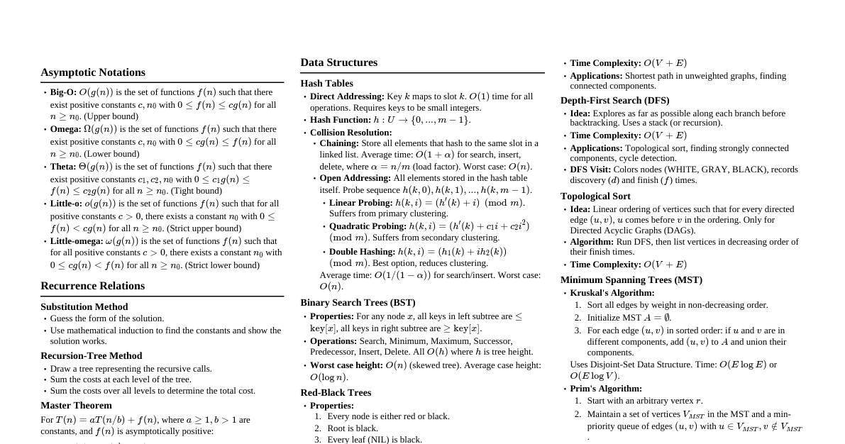
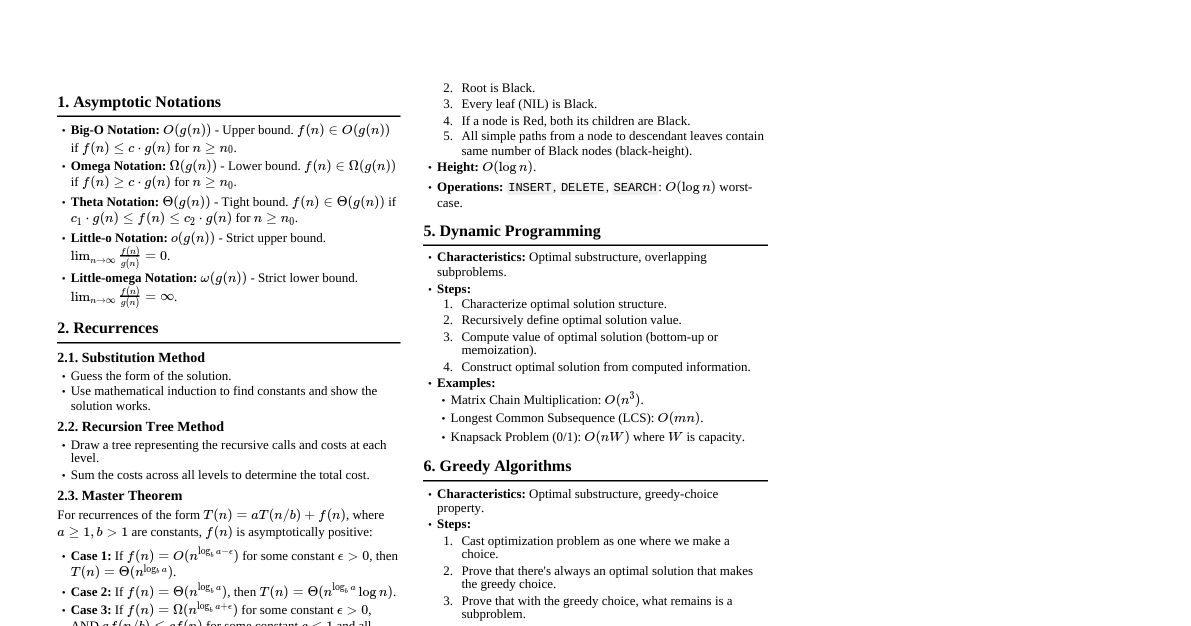
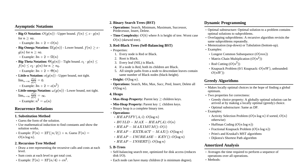
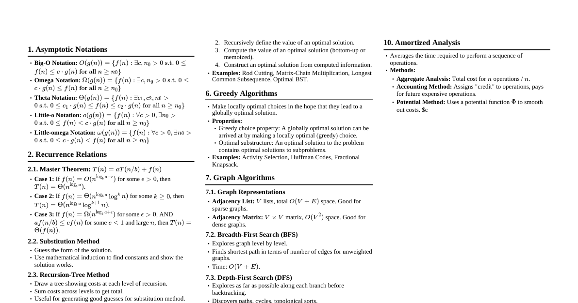
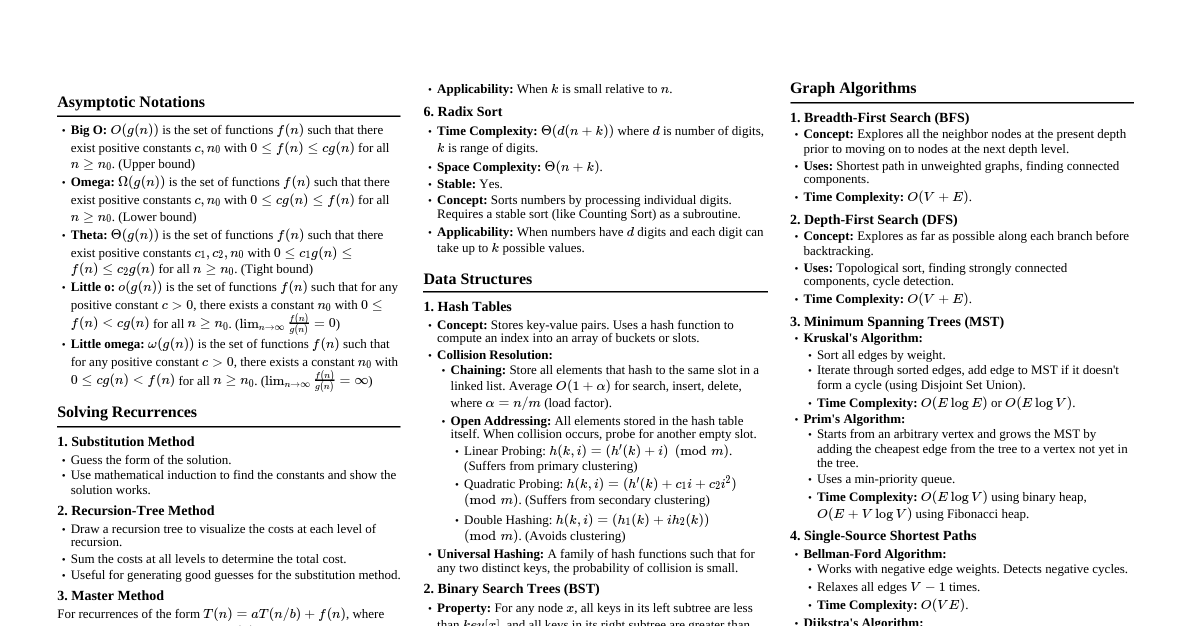
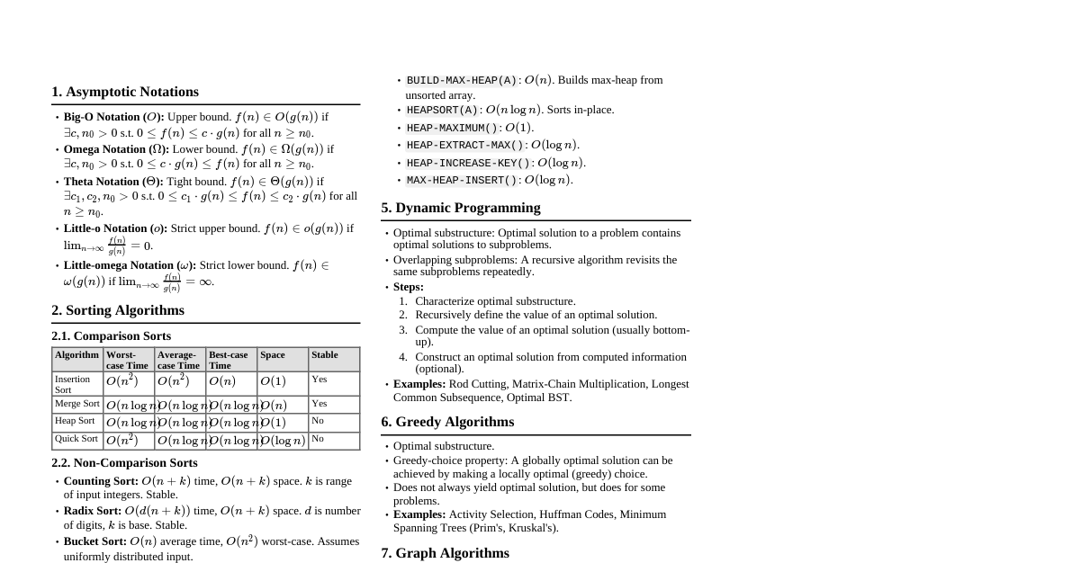
Asymptotic Notations Big O ($O(g(n))$): Upper bound. $f(n) \le c \cdot g(n)$ for $n \ge n_0$. "Worst case" growth. Big Omega ($\Omega(g(n))$): Lower bound. $f(n) \ge c \cdot g(n)$ for $n \ge n_0$. "Best case" growth. Big Theta ($\Theta(g(n))$): Tight bound. $c_1 \cdot g(n) \le f(n) \le c_2 \cdot g(n)$ for $n \ge n_0$. "Average case" growth. Little o ($o(g(n))$): $f(n)$ grows strictly slower than $g(n)$. $\lim_{n \to \infty} \frac{f(n)}{g(n)} = 0$. Little omega ($\omega(g(n))$): $f(n)$ grows strictly faster than $g(n)$. $\lim_{n \to \infty} \frac{f(n)}{g(n)} = \infty$. Recurrence Relations Substitution Method Guess a solution, then prove it by induction. Example: $T(n) = 2T(\lfloor n/2 \rfloor) + n$. Guess $T(n) = O(n \log n)$. Inductive step: Assume $T(k) \le c k \log k$ for $k Recursion Tree Method Visualize the recursion as a tree, sum costs at each level. Useful for generating educated guesses for the substitution method. Master Theorem For recurrences of the form $T(n) = aT(n/b) + f(n)$, where $a \ge 1, b > 1, f(n)$ is asymptotically positive. If $f(n) = O(n^{\log_b a - \epsilon})$ for some $\epsilon > 0$, then $T(n) = \Theta(n^{\log_b a})$. If $f(n) = \Theta(n^{\log_b a})$, then $T(n) = \Theta(n^{\log_b a} \log n)$. If $f(n) = \Omega(n^{\log_b a + \epsilon})$ for some $\epsilon > 0$, AND $a f(n/b) \le c f(n)$ for some $c Sorting Algorithms Insertion Sort Time: $O(n^2)$ worst/average, $\Omega(n)$ best. Space: $O(1)$ auxiliary. Stable: Yes. In-place: Yes. Good for small arrays or nearly sorted arrays. Merge Sort Time: $\Theta(n \log n)$ worst/average/best. Recurrence: $T(n) = 2T(n/2) + \Theta(n)$. Space: $O(n)$ auxiliary. Stable: Yes. In-place: No. Divide and conquer. Heapsort Time: $\Theta(n \log n)$ worst/average/best. Space: $O(1)$ auxiliary. Stable: No. In-place: Yes. Uses a max-heap data structure. Build-heap is $O(n)$. Quicksort Time: $O(n \log n)$ average, $O(n^2)$ worst. Recurrence: $T(n) = T(k) + T(n-k-1) + \Theta(n)$. Space: $O(\log n)$ average (recursion stack), $O(n)$ worst. Stable: No. In-place: Yes. Divide and conquer. Pivot selection is critical. Randomized Quicksort avoids worst-case. Counting Sort Time: $\Theta(n+k)$ where $k$ is range of input numbers. Space: $\Theta(n+k)$ auxiliary. Stable: Yes. Not comparison-based. Efficient for small integer ranges. Radix Sort Time: $\Theta(d(n+k))$ where $d$ is number of digits. Space: $\Theta(n+k)$ auxiliary. Stable: Yes (requires stable inner sort like Counting Sort). Sorts digits from least significant to most significant (LSD Radix Sort). Data Structures Hash Tables Average Time: $O(1)$ for insert, delete, search (with good hash function). Worst Time: $O(n)$ if all keys hash to same slot. Collision Resolution: Chaining: Each slot stores a linked list of elements. Open Addressing: Probe for next empty slot. Linear Probing: $h(k, i) = (h'(k) + i) \pmod m$. Quadratic Probing: $h(k, i) = (h'(k) + c_1 i + c_2 i^2) \pmod m$. Double Hashing: $h(k, i) = (h_1(k) + i \cdot h_2(k)) \pmod m$. Binary Search Trees (BST) Average Time: $O(h)$ for search, insert, delete ($h$ is height). $h = O(\log n)$ for balanced trees. Worst Time: $O(n)$ if tree is skewed. Properties: Left child's key Red-Black Trees Self-balancing BST. Max height $2 \log(n+1)$. Time: $O(\log n)$ for search, insert, delete. Properties: Node is Red or Black. Root is Black. Leaves (NIL) are Black. Red node has Black children. All paths from node to descendant NIL leaves contain same number of Black nodes. B-Trees Self-balancing search tree, optimized for disk access (many children per node). Time: $O(\log_t n)$ for search, insert, delete, where $t$ is minimum degree. Each node stores $t-1$ to $2t-1$ keys (except root). Fibonacci Heaps Amortized Time: Insert: $O(1)$ Minimum: $O(1)$ Extract-Min: $O(\log n)$ Decrease-Key: $O(1)$ Delete: $O(\log n)$ Union: $O(1)$ Used in algorithms like Dijkstra's and Prim's for better asymptotic bounds. Disjoint-Set Data Structure (Union-Find) Operations: Make-Set, Find-Set, Union. Amortized Time: Nearly constant, $O(\alpha(n))$ per operation with path compression and union by rank/size. ($\alpha$ is inverse Ackermann function, grows extremely slowly). Graph Algorithms Representations Adjacency List: $O(V+E)$ space. Good for sparse graphs. Adjacency Matrix: $O(V^2)$ space. Good for dense graphs, quick $O(1)$ edge lookup. Breadth-First Search (BFS) Time: $O(V+E)$. Explores level by level. Finds shortest paths in unweighted graphs. Uses a queue. Depth-First Search (DFS) Time: $O(V+E)$. Explores as deeply as possible before backtracking. Uses a stack (or recursion). Used for topological sort, strongly connected components. Topological Sort Time: $O(V+E)$. Linear ordering of vertices in a DAG where for every directed edge $(u,v)$, $u$ comes before $v$. Can be done with DFS (finish times) or by counting in-degrees. Minimum Spanning Trees (MST) Prim's Algorithm: Grows a single tree. Time: $O(E \log V)$ with binary heap, $O(E + V \log V)$ with Fibonacci heap. Kruskal's Algorithm: Grows a forest. Time: $O(E \log V)$ or $O(E \log E)$ (dominated by sorting edges). Uses Disjoint-Set. Shortest Paths Bellman-Ford Algorithm: Single-source, works with negative edge weights. Detects negative cycles. Time: $O(VE)$. Dijkstra's Algorithm: Single-source, non-negative edge weights. Time: $O(E \log V)$ with binary heap, $O(E + V \log V)$ with Fibonacci heap. Floyd-Warshall Algorithm: All-pairs shortest paths, works with negative edge weights (no negative cycles). Time: $O(V^3)$. Uses dynamic programming. Johnson's Algorithm: All-pairs shortest paths, works with negative edge weights. Time: $O(VE + V^2 \log V)$. Re-weights graph then runs Dijkstra from each vertex. Maximum Flow Ford-Fulkerson Method: Repeatedly find augmenting paths in residual graph. Time: $O(E \cdot f)$ where $f$ is max flow value (integer capacities). Can be slow. Edmonds-Karp Algorithm: Ford-Fulkerson with BFS to find augmenting paths. Time: $O(VE^2)$. Dynamic Programming Characteristics: Optimal substructure, overlapping subproblems. Approach: Characterize optimal solution's structure. Recursively define optimal solution's value. Compute value bottom-up (tabulation) or top-down with memoization. Construct an optimal solution (if needed). Examples: Rod Cutting: $R_n = \max_{1 \le i \le n} (p_i + R_{n-i})$. Matrix-Chain Multiplication: $m[i,j] = \min_{i \le k Longest Common Subsequence (LCS): If $x_i = y_j$: $c[i,j] = c[i-1,j-1] + 1$. If $x_i \ne y_j$: $c[i,j] = \max(c[i-1,j], c[i,j-1])$. Greedy Algorithms Characteristics: Optimal substructure, greedy-choice property. Approach: Make locally optimal choices hoping to reach global optimum. Examples: Activity Selection: Always pick the activity that finishes earliest. Huffman Coding: Build tree by repeatedly merging two lowest-frequency nodes. Prim's & Kruskal's MST: Local choice of minimum weight edge/connection. Dijkstra's Shortest Path: Always relax edge to closest unvisited vertex. Amortized Analysis A method for analyzing the time complexity of a sequence of operations. Aggregate Method: Total cost for $n$ operations is $T(n)$, average cost is $T(n)/n$. Accounting Method: Assign "credits" to operations, pay for cheap operations, use credits for expensive ones. Potential Method: Define a potential function $\Phi(D_i)$ for data structure state $D_i$. Amortized cost $\hat{c_i} = c_i + \Phi(D_i) - \Phi(D_{i-1})$. Example: Dynamic Array (doubling size): $O(1)$ amortized for insertions. Complexity Classes P: Problems solvable in polynomial time by a deterministic Turing machine. NP: Problems verifiable in polynomial time by a deterministic Turing machine (solution can be checked quickly). NP-Complete (NPC): Problems in NP such that every other problem in NP can be reduced to them in polynomial time. If an NPC problem can be solved in P, then P = NP. NP-Hard: Problems to which all problems in NP can be reduced in polynomial time. Need not be in NP. Co-NP: Problems whose complements are in NP. Common NPC Problems Satisfiability (SAT) 3-CNF Satisfiability (3-SAT) Clique Vertex Cover Hamiltonian Cycle Traveling Salesperson Problem (TSP) Subset Sum Knapsack Approximation Algorithms For NP-Hard problems, find a solution close to optimal within polynomial time. Approximation Ratio: If $C$ is cost of approximate solution and $C^*$ is cost of optimal, ratio is $\max(C/C^*, C^*/C)$. Example: Vertex Cover approximation (2-approximation).