Fundamentals of Electrical Engineering
Cheatsheet Content
1. DC Circuits Fundamentals 1.1 Basic Concepts Electric Current ($I$): Flow of charge. $I = dQ/dt$ (Amperes, A). Direction is conventional (positive charge flow). Voltage ($V$): Electric potential difference, energy per unit charge. $V = dW/dQ$ (Volts, V). Resistance ($R$): Opposition to current flow. $R = \rho L/A$ (Ohms, $\Omega$). $\rho$ is resistivity, $L$ is length, $A$ is cross-sectional area. Conductance ($G$): Reciprocal of resistance. $G = 1/R$ (Siemens, S). Power ($P$): Rate of energy transfer. $P = VI = I^2R = V^2/R$ (Watts, W). Energy ($W$): $W = \int P dt$ (Joules, J). 1.2 Circuit Laws Ohm's Law: $V = IR$. Relates voltage, current, and resistance in a component. Kirchhoff's Voltage Law (KVL): The algebraic sum of voltages around any closed loop in a circuit is zero. $\sum_{k=1}^N V_k = 0$. (Conservation of energy). Kirchhoff's Current Law (KCL): The algebraic sum of currents entering a node (or a closed boundary) is zero. $\sum_{k=1}^N I_k = 0$. (Conservation of charge). 1.3 Resistor Combinations Series: $R_{eq} = R_1 + R_2 + ... + R_N$. Current is same, voltage divides. Parallel: $1/R_{eq} = 1/R_1 + 1/R_2 + ... + 1/R_N$. For two resistors: $R_{eq} = (R_1 R_2) / (R_1 + R_2)$. Voltage is same, current divides. 1.4 Voltage & Current Dividers Voltage Divider Rule (VDR): For series resistors $R_1, R_2, ..., R_N$ with total voltage $V_T$, the voltage across $R_k$ is $V_{R_k} = V_T \frac{R_k}{R_1 + R_2 + ... + R_N}$. Current Divider Rule (CDR): For parallel resistors $R_1, R_2$ with total current $I_T$, the current through $R_k$ is $I_{R_k} = I_T \frac{R_{total\_parallel}}{R_k}$. For two resistors: $I_{R_1} = I_T \frac{R_2}{R_1 + R_2}$ and $I_{R_2} = I_T \frac{R_1}{R_1 + R_2}$. 1.5 Network Analysis Techniques Nodal Analysis: Apply KCL at each non-reference node. Solve for node voltages. Requires $(N-1)$ equations for $N$ nodes. Mesh Analysis: Apply KVL around each mesh (loop that does not contain any other loops). Solve for mesh currents. Requires $M$ equations for $M$ meshes. Superposition Theorem: In a linear circuit with multiple independent sources, the total response (voltage or current) in any element is the algebraic sum of the responses caused by each independent source acting alone (all other independent sources turned off). Voltage sources: Short-circuited. Current sources: Open-circuited. Thevenin's Theorem: Any linear two-terminal circuit can be replaced by an equivalent circuit consisting of a voltage source $V_{Th}$ in series with a resistor $R_{Th}$. $V_{Th}$: Open-circuit voltage across the terminals. $R_{Th}$: Equivalent resistance looking into the terminals with all independent sources turned off. Norton's Theorem: Any linear two-terminal circuit can be replaced by an equivalent circuit consisting of a current source $I_N$ in parallel with a resistor $R_N$. $I_N$: Short-circuit current between the terminals. $R_N$: Same as $R_{Th}$. Relationship: $I_N = V_{Th}/R_{Th}$. Maximum Power Transfer Theorem: Maximum power is transferred from a source to a load when the load resistance $R_L$ is equal to the Thevenin resistance $R_{Th}$ of the source network. $P_{max} = V_{Th}^2 / (4R_{Th})$. 2. DC Transients 2.1 Capacitors ($C$) Stores energy in an electric field. $Q = CV$. $I = C dV/dt$. Energy stored: $W_C = (1/2)CV^2$. Voltage across a capacitor cannot change instantaneously. In DC steady state, acts as an open circuit. 2.2 Inductors ($L$) Stores energy in a magnetic field. $V = L dI/dt$. Energy stored: $W_L = (1/2)LI^2$. Current through an inductor cannot change instantaneously. In DC steady state, acts as a short circuit. 2.3 RC Circuit (Series) Charging (connecting to DC source $V_S$): $V_C(t) = V_S(1 - e^{-t/\tau})$ $I_C(t) = (V_S/R)e^{-t/\tau}$ Time Constant $\tau = RC$. Time for voltage to reach ~63.2% of final value. Discharging (from initial voltage $V_0$): $V_C(t) = V_0 e^{-t/\tau}$ $I_C(t) = (-V_0/R)e^{-t/\tau}$ 2.4 RL Circuit (Series) Current Build-up (connecting to DC source $V_S$): $I_L(t) = (V_S/R)(1 - e^{-t/\tau})$ $V_L(t) = V_S e^{-t/\tau}$ Time Constant $\tau = L/R$. Time for current to reach ~63.2% of final value. Current Decay (from initial current $I_0$): $I_L(t) = I_0 e^{-t/\tau}$ $V_L(t) = (-I_0 R)e^{-t/\tau}$ 3. AC Fundamentals 3.1 Sinusoidal Waveforms General form: $v(t) = V_m \sin(\omega t + \phi)$ or $v(t) = V_m \cos(\omega t + \phi)$. $V_m$: Peak amplitude (max value). $\omega = 2\pi f$: Angular frequency (rad/s). $f = 1/T$: Frequency (Hz), cycles per second. $T$: Period (s), time for one complete cycle. $\phi$: Phase angle (rad or degrees), shift from reference. Phase Difference: If $v_1(t) = V_{m1} \sin(\omega t + \phi_1)$ and $v_2(t) = V_{m2} \sin(\omega t + \phi_2)$. $v_1$ leads $v_2$ if $\phi_1 > \phi_2$. $v_1$ lags $v_2$ if $\phi_1 3.2 AC Values Peak-to-Peak Value ($V_{pp}$): $2 V_m$. RMS (Root Mean Square) Value: Effective value of AC, equivalent to DC that produces same heating effect. For sine wave: $V_{rms} = V_m / \sqrt{2} \approx 0.707 V_m$. Same for current $I_{rms}$. General definition: $X_{rms} = \sqrt{\frac{1}{T}\int_0^T x^2(t) dt}$. Average Value: For a full cycle of a sine wave, average is 0. For a half-cycle: For sine wave: $V_{avg} = (2V_m)/\pi \approx 0.637 V_m$. Form Factor ($K_f$): Ratio of RMS value to Average value. $K_f = V_{rms}/V_{avg}$. For sine wave: $\pi/(2\sqrt{2}) \approx 1.11$. Peak Factor ($K_p$): Ratio of Peak value to RMS value. $K_p = V_m/V_{rms}$. For sine wave: $\sqrt{2} \approx 1.414$. 3.3 Phasor Representation Represents sinusoidal signals as complex numbers. Allows AC circuit analysis using algebraic methods. $v(t) = V_m \cos(\omega t + \phi) \leftrightarrow \mathbf{V} = V_m \angle \phi$ (Peak Phasor) Often uses RMS phasors: $v(t) = V_m \cos(\omega t + \phi) \leftrightarrow \mathbf{V} = (V_m/\sqrt{2}) \angle \phi = V_{rms} \angle \phi$. Rectangular Form: $\mathbf{Z} = R + jX$. (Real part for resistance, Imaginary part for reactance). Polar Form: $\mathbf{Z} = |\mathbf{Z}| \angle \theta$. Conversion: $R = |\mathbf{Z}| \cos\theta$, $X = |\mathbf{Z}| \sin\theta$. $|\mathbf{Z}| = \sqrt{R^2 + X^2}$, $\theta = \arctan(X/R)$. Complex Conjugate: $\mathbf{Z}^* = R - jX = |\mathbf{Z}| \angle -\theta$. 4. AC Circuit Analysis 4.1 Impedance ($Z$) Generalized resistance for AC circuits. $\mathbf{Z} = \mathbf{V}/\mathbf{I}$ (Ohms). Resistor: $\mathbf{Z}_R = R \angle 0^\circ = R$. Inductor: $\mathbf{Z}_L = j\omega L = \omega L \angle 90^\circ$. (Current lags voltage by $90^\circ$). Capacitor: $\mathbf{Z}_C = 1/(j\omega C) = -j/( \omega C) = (1/\omega C) \angle -90^\circ$. (Current leads voltage by $90^\circ$). Series Impedances: $\mathbf{Z}_{eq} = \mathbf{Z}_1 + \mathbf{Z}_2 + ...$ Parallel Impedances: $1/\mathbf{Z}_{eq} = 1/\mathbf{Z}_1 + 1/\mathbf{Z}_2 + ...$ 4.2 Admittance ($Y$) Reciprocal of impedance. $\mathbf{Y} = 1/\mathbf{Z} = G + jB$ (Siemens). $G$: Conductance (real part). $B$: Susceptance (imaginary part). Resistor: $\mathbf{Y}_R = 1/R$. Inductor: $\mathbf{Y}_L = 1/(j\omega L) = -j/( \omega L)$. Capacitor: $\mathbf{Y}_C = j\omega C$. 4.3 Power in AC Circuits Instantaneous Power: $p(t) = v(t)i(t)$. Complex Power ($\mathbf{S}$): $\mathbf{S} = \mathbf{V}\mathbf{I}^* = P + jQ$ (Volt-Amperes, VA). $\mathbf{V}$: RMS voltage phasor. $\mathbf{I}^*$: Conjugate of RMS current phasor. Magnitude $|\mathbf{S}| = V_{rms}I_{rms}$. Real Power ($P$): Average power consumed by the load. $P = V_{rms} I_{rms} \cos \phi = |\mathbf{S}| \cos \phi$ (Watts, W). $\phi$ is the angle between $\mathbf{V}$ and $\mathbf{I}$. Reactive Power ($Q$): Power exchanged between source and reactive components. $Q = V_{rms} I_{rms} \sin \phi = |\mathbf{S}| \sin \phi$ (Volt-Amperes Reactive, VAR). $Q > 0$: Inductive load (current lags voltage). $Q Apparent Power ($|\mathbf{S}|$): Total power supplied by the source. $|\mathbf{S}| = \sqrt{P^2 + Q^2}$ (VA). Power Factor (PF): $\cos \phi = P/|\mathbf{S}|$. PF = 1: Resistive load (unity PF). PF lagging: Inductive load. PF leading: Capacitive load. Power Factor Correction: Adding capacitors in parallel to inductive loads to reduce reactive power drawn from the source and improve PF. 4.4 Resonance in RLC Circuits Series RLC Circuit: Impedance: $\mathbf{Z} = R + j(\omega L - 1/(\omega C))$. Resonance occurs when $X_L = X_C$, i.e., $\omega L = 1/(\omega C)$. Resonant Frequency: $\omega_0 = 1/\sqrt{LC}$ rad/s or $f_0 = 1/(2\pi\sqrt{LC})$ Hz. At resonance: $\mathbf{Z} = R$ (minimum impedance), current is maximum, PF = 1. Quality Factor ($Q_s$): $Q_s = (\omega_0 L)/R = 1/(\omega_0 C R) = (1/R)\sqrt{L/C}$. Higher $Q_s$ means sharper resonance. Bandwidth (BW): $BW = f_0/Q_s = R/(2\pi L)$. Half-power frequencies: $f_1 = f_0 - BW/2$, $f_2 = f_0 + BW/2$. Parallel RLC Circuit: Admittance: $\mathbf{Y} = 1/R + j(\omega C - 1/(\omega L))$. Resonance occurs when $\omega C = 1/(\omega L)$. Resonant Frequency: $\omega_0 = 1/\sqrt{LC}$ rad/s or $f_0 = 1/(2\pi\sqrt{LC})$ Hz. At resonance: $\mathbf{Y} = 1/R$ (minimum admittance, maximum impedance), line current is minimum, PF = 1. Quality Factor ($Q_p$): $Q_p = R/(\omega_0 L) = \omega_0 C R = R\sqrt{C/L}$. 4.5 Three-Phase Systems Three AC voltages, typically $120^\circ$ out of phase with each other. Phase sequence: ABC (positive) or ACB (negative). Line Voltage ($V_L$): Voltage between any two lines. Phase Voltage ($V_P$): Voltage between a line and neutral (or across a phase winding). Line Current ($I_L$): Current in a line. Phase Current ($I_P$): Current through a phase winding. Star (Wye, Y) Connection: $V_L = \sqrt{3} V_P$. $I_L = I_P$. Provides a neutral point. Delta ($\Delta$) Connection: $V_L = V_P$. $I_L = \sqrt{3} I_P$. No neutral point unless created externally. Total Power (Balanced 3-Phase): Real Power: $P_{3\phi} = \sqrt{3} V_L I_L \cos \phi = 3 V_P I_P \cos \phi$. Reactive Power: $Q_{3\phi} = \sqrt{3} V_L I_L \sin \phi = 3 V_P I_P \sin \phi$. Apparent Power: $S_{3\phi} = \sqrt{3} V_L I_L = 3 V_P I_P$. 5. Magnetic Circuits & Transformers 5.1 Magnetic Circuit Concepts Magnetic Field Intensity ($H$): Force per unit magnetic pole. $H = NI/l$ (Ampere-turns/meter, A/m). Magnetic Flux Density ($B$): Amount of magnetic flux passing through a unit area perpendicular to the flux. $B = \mu H$ (Tesla, T or Wb/m$^2$). Permeability ($\mu$): Ability of a material to support the formation of a magnetic field. $\mu = \mu_0 \mu_r$. $\mu_0$: Permeability of free space ($4\pi \times 10^{-7}$ H/m). $\mu_r$: Relative permeability of the material. Magnetic Flux ($\Phi$): Total number of magnetic field lines passing through a given area. $\Phi = BA$ (Weber, Wb). Magnetomotive Force (MMF, $F$): Driving force for magnetic flux. Analogous to EMF. $F = NI$ (Ampere-turns, AT). Reluctance ($\mathcal{R}$): Opposition to the establishment of magnetic flux. $\mathcal{R} = l/(\mu A)$ (AT/Wb). Analogous to resistance. Ohm's Law for Magnetic Circuits: $F = \Phi \mathcal{R}$. Faraday's Law of Induction: $e = -N d\Phi/dt$. Induced EMF is proportional to the rate of change of magnetic flux. Lenz's Law: The direction of the induced current is such that it opposes the change in magnetic flux that produced it. Self-Inductance ($L$): $L = N\Phi/I$. Mutual Inductance ($M$): $M = N_2 \Phi_{12}/I_1$. B-H Curve (Hysteresis Loop): Plot of B vs H for a magnetic material. Shows: Saturation: Beyond a certain H, B no longer increases significantly. Retentivity ($B_r$): Residual magnetism when H is zero. Coercivity ($H_c$): Magnetic field required to demagnetize the material. Area of loop represents energy loss per cycle (hysteresis loss). 5.2 Transformers Device that transfers electrical energy from one circuit to another through electromagnetic induction, usually with a change in voltage and current. Ideal Transformer Equations: Voltage Ratio: $V_1/V_2 = N_1/N_2 = a$ (turns ratio, $a > 1$ for step-down, $a Current Ratio: $I_2/I_1 = N_1/N_2 = a$. Impedance Transformation: $Z_{in} = (N_1/N_2)^2 Z_L = a^2 Z_L$. Power: $V_1 I_1 = V_2 I_2$ (input power = output power, no losses). Practical Transformer: Includes losses and non-ideal characteristics. Losses: Core Losses: Due to alternating flux in the core. Hysteresis Loss: Energy lost in reversing magnetic domains (related to area of B-H loop). Eddy Current Loss: Circulating currents induced in the core material (reduced by laminating core). Copper Losses ($P_{cu}$): $I^2R$ losses in primary and secondary windings. $P_{cu} = I_1^2 R_1 + I_2^2 R_2$. Equivalent Circuit: Represents resistances, leakage reactances, and magnetizing branch (core losses and magnetizing reactance). Typically referred to primary or secondary side. Efficiency ($\eta$): $\eta = (P_{out} / P_{in}) \times 100\% = (P_{out} / (P_{out} + P_{losses})) \times 100\%$. Maximum efficiency occurs when copper losses equal core losses. Voltage Regulation (VR): Measures the change in secondary voltage from no-load to full-load conditions. $VR = ((V_{no-load} - V_{full-load}) / V_{full-load}) \times 100\%$. Lower VR is better. Autotransformer: A transformer with a single winding that acts as both primary and secondary. Part of the winding is common to both circuits. Advantages: Smaller size, higher efficiency, lower cost for small voltage transformations. Disadvantage: No electrical isolation between primary and secondary. Instrument Transformers: Current Transformer (CT): Steps down current for measurement. Secondary is always short-circuited. Potential Transformer (PT): Steps down voltage for measurement. Secondary is open-circuited. 6. Electrical Engineering Materials 6.1 Insulating Materials (Dielectrics) Materials that resist the flow of electric current. Properties: High dielectric strength (withstanding high voltage without breakdown), high resistivity, low dielectric loss (energy dissipated in dielectric). Applications: Cable insulation, capacitor dielectrics, transformer oil, circuit board substrates. Examples: Solid: Mica, Porcelain, PVC, Rubber, Bakelite, Paper, Glass, Ceramics. Liquid: Transformer oil, Silicone oil, Askarels (now largely banned due to toxicity). Gaseous: Air, Nitrogen, Sulphur Hexafluoride (SF6). 6.2 Conducting Materials Materials that allow electric current to flow easily. Properties: Low resistivity, high conductivity, good thermal conductivity, good mechanical strength and ductility (for wires). Applications: Wires, cables, motor/generator windings, busbars, heating elements. Examples: Copper (Cu): Excellent conductivity, ductile, corrosion resistant. Most common for wiring. Aluminum (Al): Lighter and cheaper than copper, but lower conductivity, higher resistivity, and prone to oxidation. Used for overhead lines, large cables. Silver (Ag): Highest conductivity, but expensive. Used for contacts in switches. Gold (Au): Excellent corrosion resistance, good conductivity. Used for high-reliability contacts. 6.3 Magnetic Materials Materials that can be magnetized and used to guide or store magnetic fields. Soft Magnetic Materials: Characteristics: Easily magnetized and demagnetized, narrow hysteresis loop, low coercivity, high permeability. Applications: Cores of transformers, inductors, motors, generators, relays, magnetic shielding. Examples: Silicon steel (for laminations), soft iron, ferrites (for high-frequency applications). Hard Magnetic Materials (Permanent Magnets): Characteristics: Difficult to magnetize and demagnetize, wide hysteresis loop, high retentivity, high coercivity. Applications: Permanent magnets in motors, loudspeakers, measuring instruments, memory devices. Examples: Alnico, Neodymium (NdFeB), Samarium-Cobalt (SmCo), Ferrite magnets. 6.4 Special Purpose Materials Heating Elements: Materials with high resistivity and high melting point, resistant to oxidation at high temperatures. Examples: Nichrome (Nickel-Chromium alloy), Kanthal (Iron-Chromium-Aluminum alloy). Lamp Filaments: Materials with extremely high melting point and good emissivity. Example: Tungsten. Fuses: Materials with low melting point and high resistivity to protect circuits from overcurrent. Examples: Alloys of Lead and Tin, Silver. Solders: Alloys with low melting points used to join electrical components. Examples: Lead-Tin alloys, Lead-free alloys (Tin-Silver-Copper). Thermoelectric Materials (Thermocouples): Two dissimilar metals joined at a junction. When heated, a voltage is generated (Seebeck effect). Applications: Temperature measurement. Examples: Type K (Chromel-Alumel), Type J (Iron-Constantan). Piezoelectric Materials: Generate an electric charge when mechanical stress is applied, or vice-versa. Applications: Sensors, actuators, resonators. Examples: Quartz, Barium Titanate.