알고리즘 개론 (CLRS) 핵심 정리
Cheatsheet Content
I. Foundations of Algorithm Analysis Asymptotic Notations: Describe function growth rates for large inputs. $O(g(n))$ (Big-O): Upper bound. $f(n) \le c \cdot g(n)$ for $n \ge n_0$. "At most". $\Omega(g(n))$ (Big-Omega): Lower bound. $f(n) \ge c \cdot g(n)$ for $n \ge n_0$. "At least". $\Theta(g(n))$ (Big-Theta): Tight bound. $c_1 \cdot g(n) \le f(n) \le c_2 \cdot g(n)$ for $n \ge n_0$. "Exactly". $o(g(n))$ (Little-o): Strict upper bound. $f(n)$ becomes insignificant relative to $g(n)$. $\lim_{n \to \infty} f(n)/g(n) = 0$. $\omega(g(n))$ (Little-omega): Strict lower bound. $g(n)$ becomes insignificant relative to $f(n)$. $\lim_{n \to \infty} f(n)/g(n) = \infty$. Common Growth Rates (from slowest to fastest): $\Theta(1) Summations: Arithmetic series: $\sum_{k=1}^n k = n(n+1)/2 = \Theta(n^2)$ Geometric series: $\sum_{k=0}^n r^k = (r^{n+1}-1)/(r-1)$ (for $r \ne 1$). If $0 1$, sum is $\Theta(r^n)$. Harmonic series: $\sum_{k=1}^n 1/k = \ln n + O(1) = \Theta(\log n)$ Recurrence Relations: Substitution Method: Guess a solution and prove it by induction. Recursion-Tree Method: Draw a tree, sum costs at each level, sum all levels. Master Theorem: For $T(n) = aT(n/b) + f(n)$ where $a \ge 1, b > 1$. If $f(n) = O(n^{\log_b a - \epsilon})$ for some $\epsilon > 0$, then $T(n) = \Theta(n^{\log_b a})$. If $f(n) = \Theta(n^{\log_b a})$, then $T(n) = \Theta(n^{\log_b a} \log n)$. If $f(n) = \Omega(n^{\log_b a + \epsilon})$ for some $\epsilon > 0$, AND $af(n/b) \le c f(n)$ for some $c II. Sorting Algorithms Comparison Sorts (Lower Bound $\Omega(n \log n)$): Insertion Sort: $O(n^2)$ worst/avg, $O(n)$ best. In-place, stable. Good for nearly sorted or small arrays. Merge Sort: $O(n \log n)$ always. Not in-place, stable. Recurrence: $T(n) = 2T(n/2) + \Theta(n)$. Heap Sort: $O(n \log n)$ always. In-place, not stable. Build-Heap: $O(n)$, each extraction: $O(\log n)$. Quick Sort: $O(n \log n)$ avg, $O(n^2)$ worst. In-place, not stable. Recurrence: $T(n) = T(k) + T(n-k-1) + \Theta(n)$. Worst case when partitions are unbalanced (e.g., already sorted). Non-Comparison Sorts: Counting Sort: $O(n+k)$ where $k$ is range of input integers. Not in-place, stable. Effective when $k$ is not much larger than $n$. Radix Sort: $O(d(n+k))$ where $d$ is number of digits. Not in-place, stable. Uses a stable sort (like Counting Sort) as a subroutine. Sorts digit by digit. Bucket Sort: $O(n)$ avg, $O(n^2)$ worst. Not in-place. Distributes elements into buckets, sorts each bucket (e.g., with Insertion Sort), then concatenates. Assumes input is uniformly distributed over a range. III. Data Structures Arrays: $O(1)$ access, $O(n)$ insertion/deletion (shift elements). Linked Lists: Singly, Doubly, Circular. Search: $O(n)$. Insert/Delete: $O(1)$ (if pointer to node is given), $O(n)$ (if search needed). Stacks: LIFO (Last-In, First-Out). Push, Pop $O(1)$. Queues: FIFO (First-In, First-Out). Enqueue, Dequeue $O(1)$. Hash Tables: Average $O(1)$ for search, insert, delete. Worst case $O(n)$. Collision Resolution: Chaining: Each slot points to a linked list of elements that hash to that slot. Open Addressing: Probing for next available slot (Linear, Quadratic, Double Hashing). Load Factor $\alpha = n/m$. Good performance when $\alpha \approx 1$. Binary Search Trees (BST): Search, Insert, Delete: $O(h)$ where $h$ is tree height. Worst case $O(n)$ (skewed tree), Average $O(\log n)$ (balanced tree). Red-Black Trees: (Self-balancing BST) All operations $O(\log n)$. Properties: 1. Node is Red or Black. 2. Root is Black. 3. Red node's children are Black. 4. All NIL leaves are Black. 5. All paths from a node to descendant leaves contain same number of Black nodes. B-Trees: (Generalization of BSTs for disk access) Optimized for systems that read/write large blocks of data. All leaves are at same depth. $t$ is minimum degree ($t \ge 2$). Search, Insert, Delete: $O(\log_t n)$ disk accesses. Heaps (Binary Heaps): Max-Heap / Min-Heap. Complete binary tree. Build-Heap: $O(n)$. Insert: $O(\log n)$. Max/Min-Extract: $O(\log n)$. Max/Min-Peek: $O(1)$. IV. Algorithm Design Paradigms Divide and Conquer: Divide problem into subproblems, solve recursively, combine solutions. Examples: Merge Sort, Quick Sort, Strassen's Matrix Multiplication. Dynamic Programming: Solve problems by breaking them into overlapping subproblems and storing subproblem solutions. Optimal Substructure: Optimal solution to problem contains optimal solutions to subproblems. Overlapping Subproblems: Recursive solution revisits same subproblems repeatedly. Approach: Memoization (Top-down): Store results of subproblems in a table, compute if not already there. Tabulation (Bottom-up): Fill table of solutions for subproblems from smallest to largest. Examples: Longest Common Subsequence (LCS), Matrix Chain Multiplication, 0/1 Knapsack, All-Pairs Shortest Paths (Floyd-Warshall). Greedy Algorithms: Make locally optimal choices at each step, hoping to find a globally optimal solution. Properties: Greedy-choice property, Optimal substructure. Examples: Activity Selection Problem, Huffman Coding, Minimum Spanning Tree (Kruskal, Prim). Backtracking: Explore all possible solutions by trying to build a solution incrementally. If a partial solution cannot be completed to a valid solution, abandon it (backtrack). Examples: N-Queens problem, Sudoku solver, Subset Sum. Branch and Bound: Systematically enumerates all candidate solutions for optimization problems. Uses bounds to prune search space. Examples: Traveling Salesperson Problem (TSP), Knapsack Problem. V. Graph Algorithms Graph Representations: Adjacency List: $O(V+E)$ space. Good for sparse graphs. Adjacency Matrix: $O(V^2)$ space. Good for dense graphs. Breadth-First Search (BFS): Explores layer by layer. $O(V+E)$. Finds shortest paths in unweighted graphs. Uses a queue. Depth-First Search (DFS): Explores as far as possible along each branch before backtracking. $O(V+E)$. Used for finding connected components, topological sort, strongly connected components. Uses a stack or recursion. Topological Sort: Linear ordering of vertices in a Directed Acyclic Graph (DAG) such that for every directed edge $u \to v$, $u$ comes before $v$ in the ordering. $O(V+E)$. Minimum Spanning Trees (MST): Kruskal's Algorithm: $O(E \log E)$ or $O(E \log V)$. Sort edges by weight, use Union-Find to add edges if they don't form a cycle. Prim's Algorithm: $O(E \log V)$ (binary heap) or $O(E + V \log V)$ (Fibonacci heap). Grows a single MST from a starting vertex. Single-Source Shortest Paths: Bellman-Ford Algorithm: $O(VE)$. Handles negative edge weights, detects negative cycles. Dijkstra's Algorithm: $O(E \log V)$ (binary heap) or $O(E + V \log V)$ (Fibonacci heap). Does NOT handle negative edge weights. All-Pairs Shortest Paths: Floyd-Warshall Algorithm: $O(V^3)$. Dynamic programming approach. Handles negative edge weights, detects negative cycles. Johnson's Algorithm: $O(VE + V^2 \log V)$. Reweights edges to be non-negative, then runs Dijkstra from each vertex. Good for sparse graphs. Maximum Flow: Ford-Fulkerson Method: Repeatedly finds augmenting paths in the residual graph and pushes flow. $O(E \cdot f^*)$ where $f^*$ is max flow. Edmonds-Karp Algorithm: Ford-Fulkerson with BFS to find augmenting paths. $O(VE^2)$. VI. Advanced Topics String Matching: Naive Algorithm: $O((n-m+1)m)$. Simple, but can be slow. Rabin-Karp Algorithm: $O(nm)$ worst case, $O(n+m)$ average case. Uses hashing to quickly check for matches. Knuth-Morris-Pratt (KMP) Algorithm: $O(n+m)$. Uses a precomputed "prefix function" (LPS array) to avoid redundant comparisons when a mismatch occurs. Computational Geometry: Algorithms for geometric problems (e.g., convex hull, closest pair of points, line segment intersection). Convex Hull: Smallest convex polygon enclosing a set of points. Algorithms like Graham scan ($O(n \log n)$) or Jarvis march ($O(nh)$). Number Theoretic Algorithms: Greatest Common Divisor (GCD): Euclidean Algorithm $O(\log n)$. Modular Arithmetic: Operations on integers modulo $n$. Primality Testing: Miller-Rabin (probabilistic), AKS (deterministic polynomial time). P and NP Complexity Classes: P (Polynomial time): Problems solvable in polynomial time. NP (Nondeterministic Polynomial time): Problems whose solutions can be *verified* in polynomial time. NP-Hard: Problems to which all NP problems can be reduced in polynomial time. At least as hard as any NP problem. NP-Complete: Problems that are both in NP and NP-Hard. (e.g., SAT, TSP, Hamiltonian Cycle, Vertex Cover, Knapsack). P vs NP Problem: Is P=NP? (One of the Millennium Prize Problems). Approximation Algorithms: For NP-hard optimization problems, these algorithms find near-optimal solutions in polynomial time. Performance is measured by approximation ratio. Examples: Vertex Cover, Traveling Salesperson Problem, Knapsack. Randomized Algorithms: Make random choices during execution. Las Vegas Algorithms: Always produce correct result, running time is probabilistic. (e.g., Randomized Quick Sort). Monte Carlo Algorithms: May produce incorrect result with some probability, running time is deterministic. (e.g., Miller-Rabin primality test). Linear Programming: Optimizing a linear objective function subject to linear equality and inequality constraints. Methods: Simplex Algorithm (average case polynomial, worst case exponential), Interior-Point Methods (polynomial time).
