ADSA MUSA Cheatsheet

Cheatsheet Content

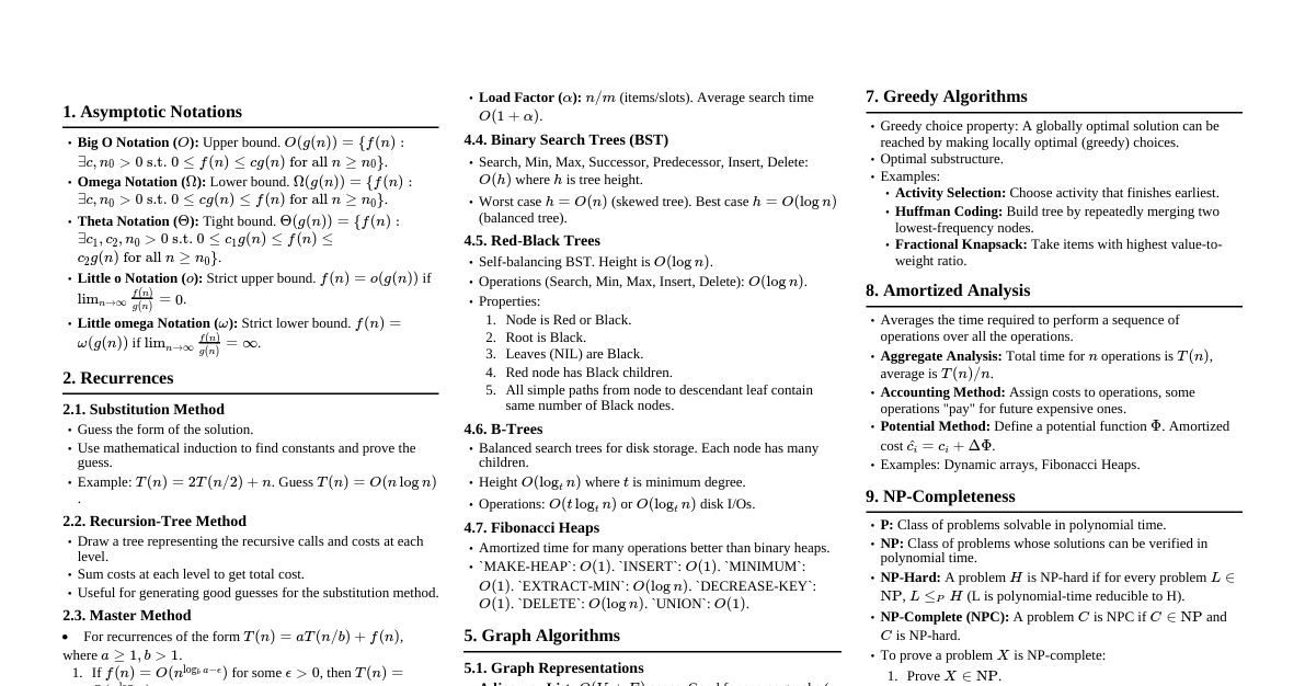
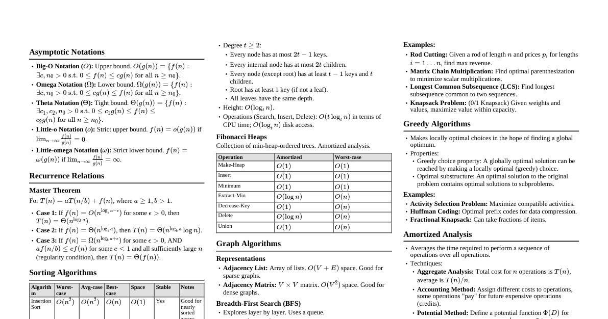
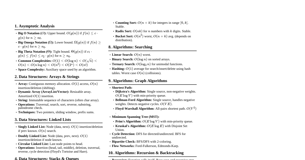
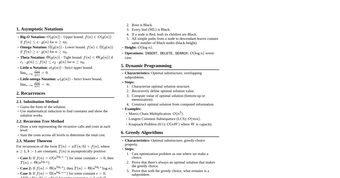
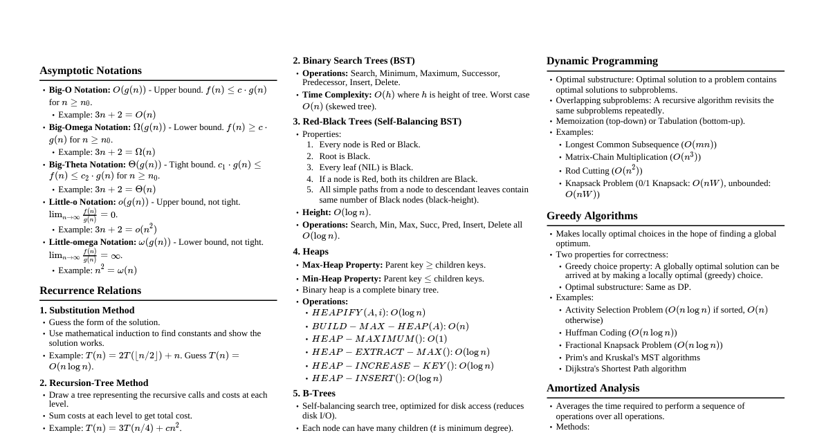
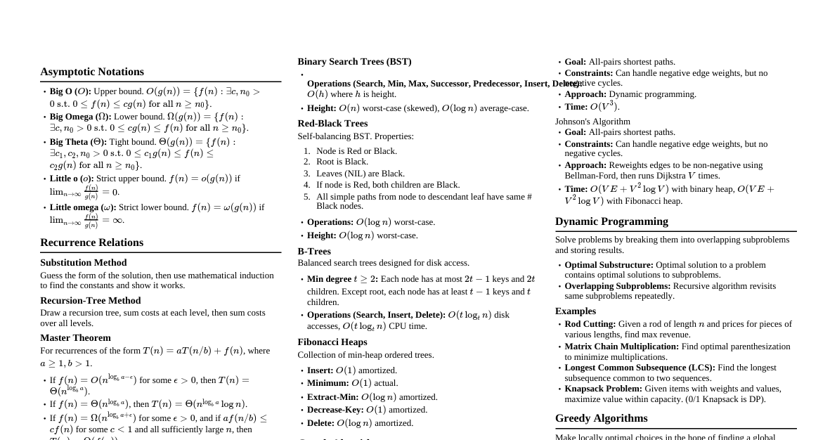
1. Introduction to Algorithms Algorithm: A precise set of instructions to solve a problem. It must be finite, definite, effective, and produce output for given input. Analysis: Evaluating an algorithm's performance (time and space complexity) using mathematical tools. Correctness: Proving an algorithm produces the correct output for all valid inputs. 2. Asymptotic Analysis: Growth of Functions Describes algorithm efficiency as input size $n$ approaches infinity, ignoring constant factors and lower-order terms. 2.1. Asymptotic Notations Big-O ($O$): Upper Bound $f(n) = O(g(n))$ if $f(n)$ grows no faster than $g(n)$. Formal: $\exists c, n_0 > 0$ such that $0 \le f(n) \le c g(n)$ for all $n \ge n_0$. Example: $3n^2 + 2n + 5 = O(n^2)$ because for $n \ge 1$, $3n^2 + 2n + 5 \le 3n^2 + 2n^2 + 5n^2 = 10n^2$ (here $c=10, n_0=1$). Big-Omega ($\Omega$): Lower Bound $f(n) = \Omega(g(n))$ if $f(n)$ grows no slower than $g(n)$. Formal: $\exists c, n_0 > 0$ such that $0 \le c g(n) \le f(n)$ for all $n \ge n_0$. Example: $3n^2 + 2n + 5 = \Omega(n^2)$ because $3n^2 + 2n + 5 \ge 3n^2$ for $n \ge 0$ (here $c=3, n_0=0$). Big-Theta ($\Theta$): Tight Bound $f(n) = \Theta(g(n))$ if $f(n)$ grows at the same rate as $g(n)$. Formal: $\exists c_1, c_2, n_0 > 0$ such that $0 \le c_1 g(n) \le f(n) \le c_2 g(n)$ for all $n \ge n_0$. Example: $3n^2 + 2n + 5 = \Theta(n^2)$ because it's both $O(n^2)$ and $\Omega(n^2)$. Little-o ($o$): Strict Upper Bound $f(n) = o(g(n))$ if $f(n)$ grows strictly slower than $g(n)$. Formal: $\forall c > 0, \exists n_0 > 0$ such that $0 \le f(n) Example: $2n = o(n^2)$. Little-omega ($\omega$): Strict Lower Bound $f(n) = \omega(g(n))$ if $f(n)$ grows strictly faster than $g(n)$. Formal: $\forall c > 0, \exists n_0 > 0$ such that $0 \le c g(n) Example: $n^2 = \omega(2n)$. 2.2. Common Time Complexities (from fastest to slowest) $O(1)$: Constant (e.g., array element access) $O(\log n)$: Logarithmic (e.g., binary search) $O(n)$: Linear (e.g., searching unsorted array) $O(n \log n)$: Log-linear (e.g., Merge Sort, Heap Sort) $O(n^2)$: Quadratic (e.g., Bubble Sort, Insertion Sort) $O(n^k)$: Polynomial (e.g., matrix multiplication) $O(2^n)$: Exponential (e.g., brute-force for TSP) $O(n!)$: Factorial (e.g., generating all permutations) 3. Divide and Conquer A recursive algorithmic paradigm that solves a problem by: Divide: Breaking the problem into smaller subproblems of the same type. Conquer: Solving the subproblems recursively. If subproblems are small enough, solve them directly. Combine: Merging the solutions of the subproblems to get the solution for the original problem. 3.1. Master Theorem for Recurrence Relations For recurrences of the form $T(n) = aT(n/b) + f(n)$, where $a \ge 1, b > 1, f(n)$ is asymptotically positive: Case 1: If $f(n) = O(n^{\log_b a - \epsilon})$ for some constant $\epsilon > 0$, then $T(n) = \Theta(n^{\log_b a})$. (The cost of the leaves dominates) Case 2: If $f(n) = \Theta(n^{\log_b a})$, then $T(n) = \Theta(n^{\log_b a} \log n)$. (Costs are balanced across levels) Case 3: If $f(n) = \Omega(n^{\log_b a + \epsilon})$ for some constant $\epsilon > 0$, AND $a f(n/b) \le c f(n)$ for some constant $c (The cost of the root dominates) 3.2. Examples Merge Sort: Divide: Split array into two halves. Conquer: Recursively sort each half. Combine: Merge the two sorted halves. Recurrence: $T(n) = 2T(n/2) + O(n)$. Here $a=2, b=2, f(n)=n$. $\log_b a = \log_2 2 = 1$. So $f(n) = \Theta(n^1)$, which matches Case 2. Time Complexity: $\Theta(n \log n)$. Space: $O(n)$ for merging. Quick Sort: Divide: Pick a pivot, partition array into elements smaller than pivot and elements larger than pivot. Conquer: Recursively sort the two partitions. Combine: No explicit combine step (sorted in place). Recurrence (Average): $T(n) = T(k) + T(n-1-k) + O(n)$. Average case $T(n) = 2T(n/2) + O(n)$. Time Complexity: Average $\Theta(n \log n)$, Worst $\Theta(n^2)$ (if pivot selection is poor, e.g., always smallest/largest). Space: $O(\log n)$ average for recursion stack, $O(n)$ worst. Binary Search: Divide: Check middle element. If not target, discard half the array. Conquer: Recursively search remaining half. Combine: Trivial. Recurrence: $T(n) = T(n/2) + O(1)$. Here $a=1, b=2, f(n)=1$. $\log_b a = \log_2 1 = 0$. So $f(n) = \Theta(n^0)$, which matches Case 2. Time Complexity: $\Theta(\log n)$. 4. Sorting Algorithms 4.1. Comparison-Based Sorts (Lower bound $\Omega(n \log n)$) Bubble Sort: Repeatedly steps through list, compares adjacent elements and swaps them if they are in the wrong order. Time: $O(n^2)$ average/worst, $O(n)$ best (already sorted). Space: $O(1)$. Stable. Insertion Sort: Builds the final sorted array (or list) one item at a time. Takes elements from input and inserts into correct position in sorted part. Time: $O(n^2)$ average/worst, $O(n)$ best. Space: $O(1)$. Stable. Efficient for small or nearly sorted arrays. Selection Sort: Repeatedly finds the minimum element from unsorted part and puts it at the beginning. Time: $O(n^2)$ always. Space: $O(1)$. Not stable. Merge Sort: (See Divide and Conquer) Time: $O(n \log n)$ always. Space: $O(n)$. Stable. Quick Sort: (See Divide and Conquer) Time: $O(n \log n)$ average, $O(n^2)$ worst. Space: $O(\log n)$ average. Not stable. Heap Sort: Uses a binary heap data structure. Builds a max-heap from input array, then repeatedly extracts max element and rebuilds heap. Time: $O(n \log n)$ always. Space: $O(1)$. Not stable. 4.2. Non-Comparison-Based Sorts (Can be faster than $O(n \log n)$ for specific data) Counting Sort: Works by counting the number of occurrences of each distinct element in the input array. Then uses these counts to determine the positions of each element in the output array. Time: $O(n+k)$ where $k$ is the range of input values. Space: $O(k)$. Stable. Best for integers with a small range. Radix Sort: Sorts integers by processing individual digits. It works by repeatedly applying a stable sorting algorithm (like counting sort) to sort the numbers by each digit position, from least significant to most significant (LSD Radix Sort) or vice-versa (MSD Radix Sort). Time: $O(d(n+k))$ where $d$ is number of digits, $k$ is base (e.g., 10 for decimal). Space: $O(n+k)$. Stable. Bucket Sort: Distributes elements into a number of buckets. Each bucket is then sorted individually (e.g., using insertion sort). Finally, the elements are gathered from the buckets in order. Time: $O(n)$ average, $O(n^2)$ worst (if all elements fall into one bucket). Space: $O(n+k)$. Best for uniformly distributed data. 5. Data Structures 5.1. Arrays Description: Contiguous block of memory storing elements of the same type. Operations: Access/Read (by index): $O(1)$. Insertion/Deletion (at arbitrary position): $O(n)$ (requires shifting elements). Insertion/Deletion (at end, if space): $O(1)$. 5.2. Linked Lists Description: Collection of nodes where each node contains data and a pointer to the next node. Not contiguous in memory. Types: Singly, Doubly (pointers to next and previous), Circular. Operations: Access/Search: $O(n)$. Insertion/Deletion: $O(1)$ (if pointer to the node is given, otherwise $O(n)$ to find node). 5.3. Stacks (LIFO - Last-In, First-Out) Description: Abstract data type. Operations happen at one end (top). Operations: push(item) : Add item to top. $O(1)$. pop() : Remove item from top. $O(1)$. peek() : Get top item without removing. $O(1)$. isEmpty() : Check if stack is empty. $O(1)$. Applications: Function call stack, expression evaluation, undo/redo. 5.4. Queues (FIFO - First-In, First-Out) Description: Abstract data type. Operations happen at two ends (front and rear). Operations: enqueue(item) : Add item to rear. $O(1)$. dequeue() : Remove item from front. $O(1)$. front() : Get front item without removing. $O(1)$. isEmpty() : Check if queue is empty. $O(1)$. Applications: Task scheduling, BFS, printer queues. 5.5. Trees Non-linear data structure with a root node and child nodes. Binary Tree: Each node has at most two children (left and right). Binary Search Tree (BST): Left child's value $\le$ parent's value $\le$ right child's value. Operations: Search, Insert, Delete. $O(h)$ where $h$ is tree height. Average case: $O(\log n)$ (for balanced tree). Worst case: $O(n)$ (for skewed tree). Self-Balancing BSTs (AVL, Red-Black Trees): Maintain $O(\log n)$ height to guarantee $O(\log n)$ for all operations. AVL Tree: For every node, the height difference between left and right subtrees is at most 1. Uses rotations to rebalance. Red-Black Tree: More relaxed balancing rules, but still guarantees $O(\log n)$ height. Properties: Node is Red or Black. Root is Black. No two adjacent Red nodes (Red node cannot have Red child). Every path from a node to any of its descendant NIL nodes has the same number of Black nodes. B-Tree: Designed for disk-based storage (minimizes disk I/O). Nodes can have many children (order $m$). All leaves are at the same depth. Nodes store keys in sorted order. Operations: Search, Insert, Delete. $O(\log_t N)$ where $t$ is minimum degree of node (related to $m$). 5.6. Heaps Description: A complete binary tree that satisfies the heap property. Heap Property: Max-Heap: For every node $i$ other than the root, $A[parent(i)] \ge A[i]$. (Largest element at root) Min-Heap: For every node $i$ other than the root, $A[parent(i)] \le A[i]$. (Smallest element at root) Operations: insert(item) : Add to end, then "heapify-up". $O(\log n)$. extractMax()/extractMin() : Remove root, replace with last element, then "heapify-down". $O(\log n)$. buildHeap(array) : Convert an array into a heap. $O(n)$. Applications: Priority Queues, Heap Sort. 5.7. Hash Tables Description: Data structure that maps keys to values using a hash function. Provides fast average-case lookups. Hash Function: Maps keys to indices in an array (hash table/bucket array). Collisions: When two different keys hash to the same index. Collision Resolution Strategies: Chaining: Store a linked list of elements at each array index. Open Addressing: If a slot is taken, probe for another slot (linear probing, quadratic probing, double hashing). Operations: Insert, Delete, Search: Average $O(1)$, Worst case $O(n)$ (if many collisions result in a long chain or probe sequence). 5.8. Graphs Description: A set of vertices (nodes) $V$ and a set of edges (connections) $E$. $G = (V, E)$. Types: Directed/Undirected, Weighted/Unweighted, Cyclic/Acyclic (DAG - Directed Acyclic Graph). Representations: Adjacency Matrix: An $V \times V$ matrix where $A[i][j]$ indicates presence/weight of edge between $V_i$ and $V_j$. Space $O(V^2)$. Fast for checking edge existence. Adjacency List: An array of linked lists where $adj[i]$ contains a list of vertices adjacent to $V_i$. Space $O(V+E)$. Efficient for sparse graphs. Graph Traversal: Breadth-First Search (BFS): Explores layer by layer. Uses a Queue. Algorithm: Start at source $s$, visit $s$, enqueue $s$. While queue not empty, dequeue $u$, visit all unvisited neighbors of $u$, mark visited, enqueue them. Time: $O(V+E)$. Used for shortest path in unweighted graphs, finding connected components. Depth-First Search (DFS): Explores as far as possible along each branch before backtracking. Uses a Stack (or recursion). Algorithm: Start at source $s$, visit $s$, push $s$ to stack. While stack not empty, pop $u$, for each unvisited neighbor $v$ of $u$, visit $v$, push $v$ to stack. Time: $O(V+E)$. Used for topological sort, finding connected components, cycle detection. Minimum Spanning Tree (MST): A subgraph of a connected, edge-weighted undirected graph that connects all the vertices together, without any cycles and with the minimum possible total edge weight. Prim's Algorithm: Grows the MST from an arbitrary starting vertex. At each step, adds the cheapest edge connecting a vertex in the MST to a vertex outside the MST. Uses a min-priority queue. Time: $O(E \log V)$ with binary heap, $O(E+V \log V)$ with Fibonacci heap. Kruskal's Algorithm: Sorts all edges by weight in non-decreasing order. Iterates through sorted edges, adding an edge to the MST if it does not form a cycle with already added edges. Uses Disjoint Set Union (DSU) data structure to detect cycles efficiently. Time: $O(E \log E)$ or $O(E \log V)$ (since $E \le V^2$, $\log E$ is $2 \log V$). Shortest Path Algorithms: Dijkstra's Algorithm: Single-source shortest paths for graphs with non-negative edge weights. Uses a min-priority queue to always extract the unvisited vertex with the smallest known distance. Time: $O(E \log V)$ with binary heap, $O(E+V \log V)$ with Fibonacci heap. Bellman-Ford Algorithm: Single-source shortest paths for graphs with potentially negative edge weights. Can detect negative cycles. Relaxes all edges $V-1$ times. If a path can still be relaxed in the $V$-th iteration, a negative cycle exists. Time: $O(VE)$. Floyd-Warshall Algorithm: All-pairs shortest paths for graphs with positive or negative edge weights (no negative cycles). Dynamic Programming approach: $dist[i][j][k]$ is shortest path from $i$ to $j$ using intermediate vertices from $\{1, \dots, k\}$. Time: $O(V^3)$. A* Search Algorithm: Finds shortest path in a graph using a heuristic function $h(n)$ to estimate cost from $n$ to goal. Evaluates nodes based on $f(n) = g(n) + h(n)$, where $g(n)$ is cost from start to $n$. If $h(n)$ is admissible (never overestimates), A* finds optimal path. Time: Depends on heuristic; can be exponential in worst case, but often much faster. Topological Sort: A linear ordering of vertices in a Directed Acyclic Graph (DAG) such that for every directed edge $u \to v$, vertex $u$ comes before vertex $v$ in the ordering. Kahn's Algorithm: Uses in-degrees of vertices and a queue. Compute in-degree for all vertices. Enqueue all vertices with in-degree 0. While queue not empty: Dequeue $u$, add $u$ to topological order. For each neighbor $v$ of $u$, decrement in-degree of $v$. If in-degree of $v$ becomes 0, enqueue $v$. DFS-based Algorithm: Perform DFS. When a vertex finishes (all its descendants visited), add it to the front of a list. Time: $O(V+E)$. 6. Dynamic Programming An optimization technique for problems with overlapping subproblems and optimal substructure . Overlapping Subproblems: A recursive algorithm revisits the same subproblems repeatedly. DP solves each subproblem once and stores its result. Optimal Substructure: An optimal solution to the problem contains optimal solutions to its subproblems. Approaches: Memoization (Top-down): Recursive approach. Solve subproblems as needed, store results in a table (e.g., array or hash map). If result for subproblem already computed, return it. Tabulation (Bottom-up): Iterative approach. Solve all "smaller" subproblems first, then use their solutions to build solutions for larger subproblems. Fills a table iteratively. 6.1. Examples Fibonacci Sequence: $F(n) = F(n-1) + F(n-2)$, $F(0)=0, F(1)=1$. Naive recursion: $O(2^n)$ due to recomputing. Memoization: Store $F(i)$ in an array. $O(n)$ time, $O(n)$ space. Tabulation: Iterate from $i=2$ to $n$, computing $F(i) = F(i-1) + F(i-2)$. $O(n)$ time, $O(n)$ space (can be $O(1)$ space). Longest Common Subsequence (LCS): Given two sequences, find the longest subsequence common to both. Let $dp[i][j]$ be the length of LCS of $X[1 \dots i]$ and $Y[1 \dots j]$. If $X[i] == Y[j]$, then $dp[i][j] = 1 + dp[i-1][j-1]$. Else, $dp[i][j] = \max(dp[i-1][j], dp[i][j-1])$. Time: $O(mn)$ for sequences of length $m, n$. Space: $O(mn)$. 0/1 Knapsack Problem: Given $n$ items, each with a weight $w_i$ and value $v_i$, and a knapsack capacity $W$. Choose a subset of items to maximize total value, such that total weight does not exceed $W$. Each item can be taken or not (0/1). Let $dp[i][w]$ be max value using first $i$ items with capacity $w$. $dp[i][w] = dp[i-1][w]$ (if item $i$ not taken) $dp[i][w] = \max(dp[i-1][w], v_i + dp[i-1][w-w_i])$ (if item $i$ taken, if $w_i \le w$). Time: $O(nW)$. Space: $O(nW)$ (can be optimized to $O(W)$). Matrix Chain Multiplication: Given a sequence of matrices, find the most efficient way to multiply them. The problem is to parenthesize the product. $dp[i][j]$ = minimum number of scalar multiplications needed to compute product $A_i A_{i+1} \dots A_j$. Time: $O(n^3)$. Space: $O(n^2)$. 7. Greedy Algorithms Makes the locally optimal choice at each step, hoping this leads to a globally optimal solution. Properties for correctness: Greedy Choice Property: A globally optimal solution can be achieved by making a locally optimal (greedy) choice. Optimal Substructure: An optimal solution to the overall problem contains optimal solutions to subproblems. Not all optimization problems can be solved correctly by a greedy approach. 7.1. Examples Activity Selection Problem: Given a set of activities, each with a start and finish time, select the maximum number of non-overlapping activities. Greedy Strategy: Sort activities by their finish times. Always pick the activity that finishes earliest among the compatible ones. Time: $O(n \log n)$ for sorting, then $O(n)$ for selection. Fractional Knapsack Problem: Items can be taken partially. Maximize value within capacity $W$. Greedy Strategy: Calculate value-to-weight ratio ($v_i/w_i$) for each item. Sort items by this ratio in descending order. Take items with highest ratio first, taking fractions if needed. Time: $O(n \log n)$ for sorting. Huffman Coding: Builds an optimal prefix code for data compression. Greedy Strategy: Repeatedly merge the two nodes (characters or subtrees) with the smallest frequencies until one tree remains. Uses a min-priority queue. Time: $O(N \log N)$ where $N$ is number of distinct characters. Dijkstra's, Prim's, Kruskal's Algorithms: Are all greedy algorithms. 8. Backtracking An algorithmic technique for solving problems recursively by trying to build a solution incrementally, one piece at a time. When a partial solution is found that cannot possibly be completed to a valid solution, the algorithm "backtracks" to an earlier state and tries a different option. Explores all possible paths/solutions. Often implemented with recursion. 8.1. Examples N-Queens Problem: Place $N$ non-attacking queens on an $N \times N$ chessboard. Algorithm: Start with an empty board. Place a queen in the first row. For each subsequent row, try to place a queen in a column that is not attacked by previously placed queens. If no safe column is found, backtrack to the previous row and try a different column for that queen. Sudoku Solver: Fill a $9 \times 9$ grid following Sudoku rules. Finding all Hamiltonian Cycles in a graph. Subset Sum Problem: Find a subset of a given set of numbers that sums to a target value. 9. Branch and Bound An algorithm design paradigm for optimization problems, often more efficient than pure backtracking. Systematically explores a tree of possible solutions (like backtracking). Uses "bounding" functions to prune branches of the search tree that cannot possibly contain an optimal solution. This reduces the search space. Components: Branching: Dividing the problem into subproblems. Bounding: Calculating an upper/lower bound for the optimal solution in each subproblem. If a subproblem's bound is worse than a known global optimal, it's pruned. 9.1. Examples Traveling Salesperson Problem (TSP): Find the shortest possible route that visits each city exactly once and returns to the origin city. 0/1 Knapsack Problem: Can be solved with Branch and Bound for exact solutions. 10. Complexity Classes Categorizing computational problems based on the resources required to solve them. P (Polynomial Time): Class of decision problems (yes/no answer) solvable by a deterministic Turing machine in polynomial time ($O(n^k)$ for some constant $k$). Considered "efficiently solvable". Examples: Sorting, searching, MST, shortest path (Dijkstra's). NP (Nondeterministic Polynomial Time): Class of decision problems for which a given solution (certificate) can be *verified* in polynomial time by a deterministic Turing machine. Does NOT mean "not polynomial". Many NP problems are solvable in polynomial time (all P problems are also NP). Examples: Satisfiability, Hamiltonian cycle, TSP (decision version). NP-Hard: A problem $H$ is NP-hard if for every problem $L$ in NP, there is a polynomial-time reduction from $L$ to $H$. This means $H$ is at least as hard as any problem in NP. An NP-hard problem may not be in NP itself (e.g., it might be an optimization problem, not a decision problem). NP-Complete (NPC): A problem $C$ is NP-complete if $C$ is in NP AND $C$ is NP-hard. These are the "hardest" problems in NP. If any NP-complete problem can be solved in polynomial time, then all problems in NP can be solved in polynomial time (i.e., P=NP). Examples: Boolean Satisfiability Problem (SAT), Clique, Vertex Cover, Hamiltonian Cycle, Traveling Salesperson Problem (decision version). The P vs. NP Problem: Whether P=NP (Can every problem whose solution can be quickly verified also be quickly solved?) is one of the most important unsolved problems in theoretical computer science. Most computer scientists believe P $\ne$ NP. 11. Amortized Analysis A method for analyzing the time complexity of an algorithm or data structure operations, where a sequence of operations is considered rather than focusing on the worst-case time of a single operation. It provides an average performance guarantee over a sequence of operations, even if some individual operations are very expensive. Methods: Aggregate Analysis: Sum up total cost of $n$ operations, then divide by $n$. Accounting Method: Assign "credits" to operations; some operations are "overcharged" to pay for future expensive operations. Potential Method: Define a potential function $\Phi$ for the data structure. Amortized cost $\hat{c_i} = c_i + \Delta\Phi_i$. 11.1. Example: Dynamic Array (e.g., `ArrayList` in Java, `list` in Python) Operation: `append()` Most appends take $O(1)$ time (just add to end). When the array is full, a new, larger array (e.g., double the size) is allocated, and all elements are copied from the old array to the new one. This takes $O(n)$ time, where $n$ is the current number of elements. If we just consider worst-case, `append()` is $O(n)$. Amortized Analysis: Over a sequence of $n$ appends starting with an empty array, the total cost for copying elements is $O(n)$. Thus, the amortized cost per append operation is $O(n)/n = O(1)$. 12. String Matching Algorithms Finding occurrences of a "pattern" string $P$ within a "text" string $T$. Let $|T|=n, |P|=m$. Naive String Matching: Compares the pattern with all possible $n-m+1$ shifts of the pattern relative to the text. Time: $O((n-m+1)m)$, worst case $O(nm)$. (e.g., $P = \text{"aaa"}, T = \text{"aaaaa"}$) Rabin-Karp Algorithm: Uses hashing to quickly filter out impossible shifts. A hash value is computed for the pattern and for each $m$-character window in the text. If hash values match, then a character-by-character comparison is done to confirm. Uses a "rolling hash" to efficiently compute hash for next window. Time: Average $O(n+m)$, Worst case $O(nm)$ (if many spurious matches due to poor hash function). Knuth-Morris-Pratt (KMP) Algorithm: Avoids re-examining characters of text $T$ that have already been matched. Preprocesses the pattern $P$ to build a "Longest Proper Prefix Suffix" (LPS) array (also called "failure function"). This array tells how many characters to shift the pattern when a mismatch occurs. Time: $O(n+m)$ (Preprocessing LPS array: $O(m)$, Matching: $O(n)$). Boyer-Moore Algorithm: Often very fast in practice, especially for long patterns and alphabet. Compares pattern from right-to-left. Uses two heuristics to determine shift amount: Bad Character Heuristic: If a mismatch occurs, shift pattern so that the mismatched character in text aligns with its last occurrence in pattern (or shifts past pattern if not present). Good Suffix Heuristic: If a suffix of pattern matches, but preceding character mismatches, shift pattern to align with another occurrence of that good suffix. Time: Worst case $O(nm)$, but often sublinear $O(n/m)$ in practice. 13. Graph Algorithms (Advanced) 13.1. Flow Networks Flow Network: A directed graph where each edge has a capacity, and each edge can carry a certain amount of "flow". Source $s$ (only outgoing flow), Sink $t$ (only incoming flow). Max-Flow Problem: Find the maximum possible flow from $s$ to $t$. Min-Cut Problem: Find a partition of vertices into two sets $(S, T)$ such that $s \in S, t \in T$, and the sum of capacities of edges going from $S$ to $T$ is minimized. Max-Flow Min-Cut Theorem: The value of a maximum flow is equal to the capacity of a minimum cut. Ford-Fulkerson Algorithm: Iteratively finds "augmenting paths" (paths from $s$ to $t$ in the residual graph with available capacity) and pushes flow along them until no more augmenting paths can be found. Time: $O(E \cdot f_{max})$ where $f_{max}$ is max flow value (can be slow if capacities are large). Edmonds-Karp Algorithm: A specific implementation of Ford-Fulkerson that uses BFS to find shortest augmenting paths (in terms of number of edges). Time: $O(VE^2)$. Dinic's Algorithm: More advanced max-flow algorithm. Uses BFS to construct a "level graph" (or "layered network") and then uses DFS to find "blocking flows" (maximal flow along disjoint paths in the level graph). Time: $O(V^2 E)$ in general graphs, $O(V E^2)$ for unit capacities, $O(E \min(V^{2/3}, E^{1/2}))$ for unit networks. 13.2. Bipartite Matching Bipartite Graph: A graph whose vertices can be divided into two disjoint and independent sets $U$ and $V$ such that every edge connects a vertex in $U$ to one in $V$. Matching: A set of edges such that no two edges share a common vertex. Maximum Matching: A matching with the largest possible number of edges. Algorithm: Can be solved by transforming into a max-flow problem: Create a source $s$ and a sink $t$. Add edges from $s$ to all vertices in $U$ with capacity 1. Add edges from all vertices in $V$ to $t$ with capacity 1. For every edge $(u, v)$ in the original bipartite graph ($u \in U, v \in V$), add a directed edge from $u$ to $v$ with capacity 1. The max flow in this network equals the size of the maximum matching. Hopcroft-Karp Algorithm: A dedicated algorithm for maximum bipartite matching. Time: $O(E \sqrt{V})$. 14. Geometric Algorithms Convex Hull: The smallest convex polygon that contains a given set of points in a 2D plane. Graham Scan: Find the lowest point (and leftmost if tie). This point is definitely on the hull. Sort all other points by angle they make with the lowest point. Iterate through sorted points, maintaining a stack. For each point, pop points from stack that would create a non-left turn (non-convex angle) with the current point. Push current point. Time: $O(N \log N)$ (dominated by sorting). Jarvis March (Gift Wrapping): Find the lowest point $P_0$. Add $P_0$ to hull. From current hull point $P_i$, find the next point $P_{i+1}$ such that $P_{i+1}$ makes the smallest counter-clockwise angle with $P_i$ and the previous hull point (or horizontal axis). Repeat until $P_0$ is reached again. Time: $O(Nh)$ where $h$ is the number of points on the convex hull. Can be $O(N^2)$ in worst case ($h=N$). Closest Pair of Points: Given a set of $N$ points in a 2D plane, find the two points that are closest to each other. Divide and Conquer: Sort points by x-coordinate. Divide the set into two halves, $P_L$ and $P_R$, by a vertical line. Recursively find closest pair in $P_L$ (distance $d_L$) and $P_R$ (distance $d_R$). Let $d = \min(d_L, d_R)$. Consider points in a "strip" of width $2d$ around the dividing line. Sort these points by y-coordinate. Check distances for points within this strip (at most 7 points need to be checked for each point). Time: $O(N \log N)$.