DSA Essentials
Cheatsheet Content
1. Asymptotic Analysis Big O Notation ($O$): Upper bound, worst-case. $O(1)$: Constant time $O(\log n)$: Logarithmic time $O(n)$: Linear time $O(n \log n)$: Linearithmic time $O(n^2)$: Quadratic time $O(2^n)$: Exponential time $O(n!)$: Factorial time Omega Notation ($\Omega$): Lower bound, best-case. Theta Notation ($\Theta$): Tight bound, average-case. 2. Data Structures 2.1. Arrays Definition: Contiguous memory allocation. Access: $O(1)$ by index. Insertion/Deletion: $O(n)$ in general (needs shifting). Operations: Lookup: $O(1)$ Insert at end: $O(1)$ amortized Insert at middle/beginning: $O(n)$ Delete: $O(n)$ 2.2. Linked Lists Definition: Nodes with data and a pointer to the next node. Types: Singly: Node $\rightarrow$ Node $\rightarrow$ Null Doubly: Null $\leftarrow$ Node $\leftrightarrow$ Node $\rightarrow$ Null Circular: Last node points to first. Operations: Access: $O(n)$ Insertion/Deletion: $O(1)$ (if position known), $O(n)$ (if search needed) 2.3. Stacks Definition: LIFO (Last In, First Out) structure. Operations: push(item) : Add item to top ($O(1)$). pop() : Remove item from top ($O(1)$). peek() : View top item ($O(1)$). isEmpty() : Check if stack is empty ($O(1)$). Applications: Function calls, undo/redo, expression evaluation. 2.4. Queues Definition: FIFO (First In, First Out) structure. Operations: enqueue(item) : Add item to rear ($O(1)$). dequeue() : Remove item from front ($O(1)$). front() : View front item ($O(1)$). isEmpty() : Check if queue is empty ($O(1)$). Applications: Task scheduling, breadth-first search. 2.5. Hash Tables (Hash Maps) Definition: Stores key-value pairs using a hash function. Average Operations: $O(1)$ for insert, delete, lookup. Worst-Case Operations: $O(n)$ (due to collisions). Collision Resolution: Chaining: Linked list at each bucket. Open Addressing: Linear probing, quadratic probing, double hashing. 2.6. Trees Definition: Non-linear data structure with a root, nodes, and children. Terminology: Root, parent, child, sibling, leaf, depth, height. Binary Tree: Each node has at most two children. Binary Search Tree (BST): Left child Average Time: $O(\log n)$ for search, insert, delete. Worst-Case Time: $O(n)$ (skewed tree). Balanced BSTs (AVL, Red-Black Trees): Guarantee $O(\log n)$ operations. Heaps: Complete binary tree satisfying heap property. Max-Heap: Parent $\ge$ children. Min-Heap: Parent $\le$ children. Operations: insert ($O(\log n)$), deleteMax/Min ($O(\log n)$), heapify ($O(n)$). Applications: Priority queues, Heap Sort. Tries (Prefix Trees): Efficient for string operations (e.g., autocomplete). 2.7. Graphs Definition: Set of vertices (nodes) and edges (connections). Terminology: Vertex, Edge, Directed/Undirected, Weighted/Unweighted, Cycle, Path, Degree. Representations: Adjacency Matrix: $A[i][j]=1$ if edge $(i,j)$ exists. $O(V^2)$ space. Adjacency List: Array of linked lists. $O(V+E)$ space. 3. Algorithms 3.1. Sorting Algorithms Algorithm Time Complexity (Avg) Time Complexity (Worst) Space Complexity Bubble Sort $O(n^2)$ $O(n^2)$ $O(1)$ Selection Sort $O(n^2)$ $O(n^2)$ $O(1)$ Insertion Sort $O(n^2)$ $O(n^2)$ $O(1)$ Merge Sort $O(n \log n)$ $O(n \log n)$ $O(n)$ Quick Sort $O(n \log n)$ $O(n^2)$ $O(\log n)$ (avg) Heap Sort $O(n \log n)$ $O(n \log n)$ $O(1)$ 3.2. Searching Algorithms Linear Search: Traverse array sequentially. $O(n)$ time. Binary Search: For sorted arrays, repeatedly divide search interval in half. $O(\log n)$ time. 3.3. Graph Traversal Algorithms Breadth-First Search (BFS): Uses a queue. Explores level by level. Finds shortest path in unweighted graphs. Time: $O(V+E)$. Depth-First Search (DFS): Uses a stack (or recursion). Explores as far as possible along each branch. Applications: Topological sort, cycle detection. Time: $O(V+E)$. 3.4. Shortest Path Algorithms Dijkstra's Algorithm: Finds shortest paths from a single source to all other vertices in a non-negative weighted graph. Uses a min-priority queue. Time: $O(E \log V)$ or $O(E + V \log V)$ with Fibonacci heap. Bellman-Ford Algorithm: Finds shortest paths from a single source in a weighted graph, can handle negative edge weights. Detects negative cycles. Time: $O(VE)$. Floyd-Warshall Algorithm: Finds all-pairs shortest paths in a weighted graph. Time: $O(V^3)$. 3.5. Minimum Spanning Tree (MST) Algorithms Prim's Algorithm: Builds an MST by adding edges one by one to a growing tree. Starts from an arbitrary vertex. Time: $O(E \log V)$ or $O(E + V \log V)$ with Fibonacci heap. Kruskal's Algorithm: Builds an MST by adding the cheapest available edge that doesn't form a cycle. Uses a Disjoint Set Union (DSU) data structure. Time: $O(E \log E)$ or $O(E \log V)$. 4. Algorithmic Paradigms Brute Force: Tries all possible solutions. Divide and Conquer: Break problem into smaller subproblems. Solve subproblems recursively. Combine solutions. Examples: Merge Sort, Quick Sort. Greedy Algorithms: Makes locally optimal choices at each step with the hope of finding a global optimum. Examples: Dijkstra's, Prim's, Kruskal's. Dynamic Programming: Solves problems by breaking them into overlapping subproblems and storing results of subproblems to avoid recomputation. Memoization: Top-down (recursive with cache). Tabulation: Bottom-up (iterative with table). Examples: Fibonacci, Longest Common Subsequence. Backtracking: Explores all potential solutions incrementally, abandoning paths that cannot lead to a valid solution. Uses recursion. Examples: N-Queens, Sudoku Solver. 5. Common Techniques Two Pointers: Efficiently traverse arrays/lists. Sliding Window: Used for contiguous subarrays/substrings. Recursion: Function calls itself. Base case: Termination condition. Recursive step: Call with smaller input. Iteration: Loops (for, while).