Introduction to Algorithms (CLRS)

Cheatsheet Content

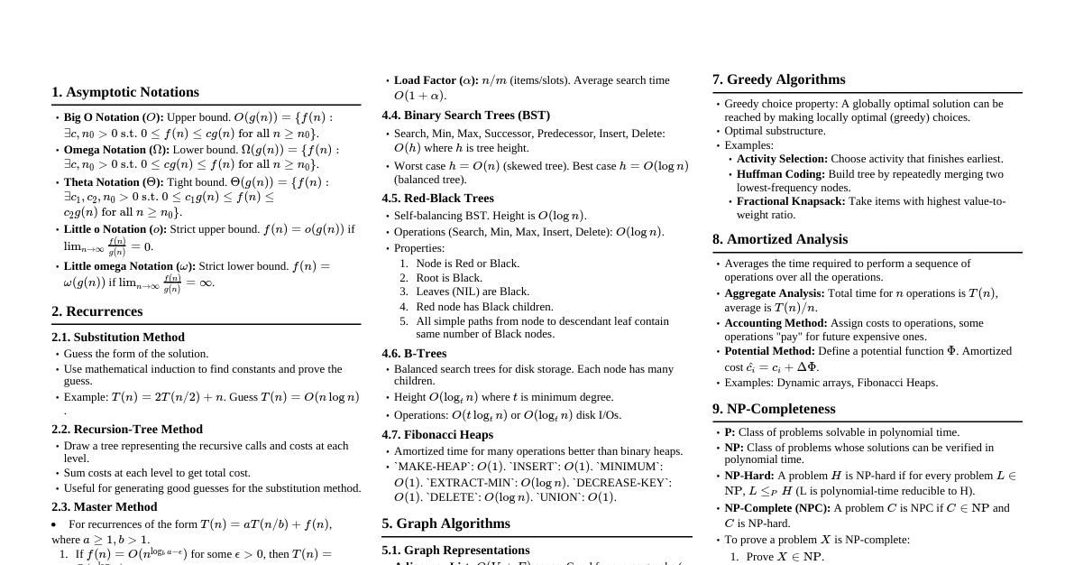
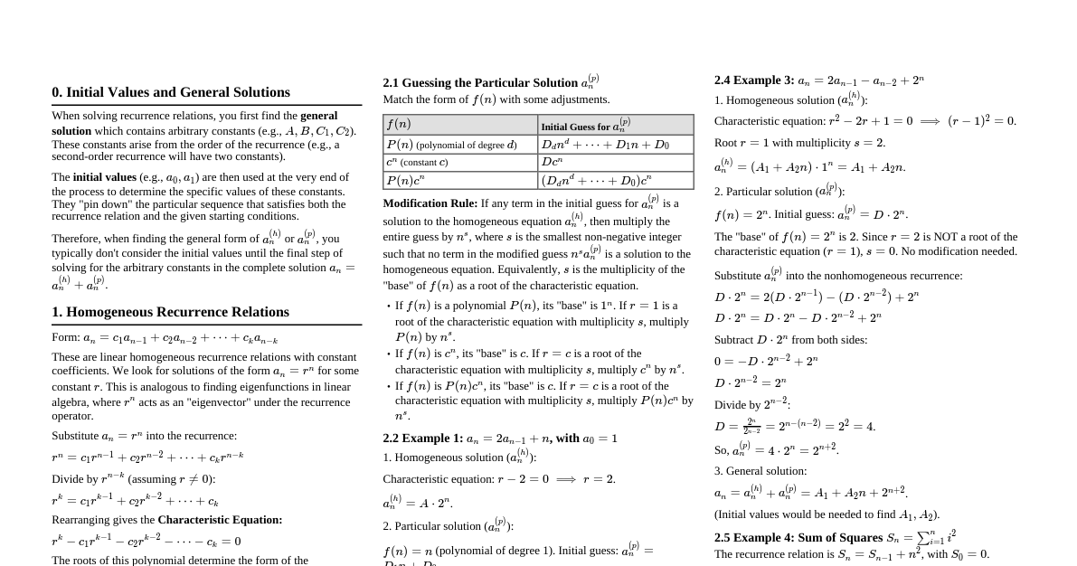
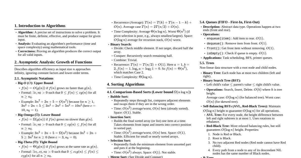
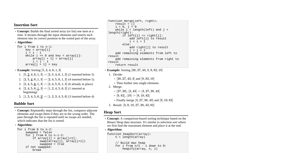
Asymptotic Notations Big O ($O$): Upper bound. $O(g(n)) = \{f(n) : \exists c, n_0 > 0 \text{ s.t. } 0 \le f(n) \le c g(n) \text{ for all } n \ge n_0\}$. Big Omega ($\Omega$): Lower bound. $\Omega(g(n)) = \{f(n) : \exists c, n_0 > 0 \text{ s.t. } 0 \le c g(n) \le f(n) \text{ for all } n \ge n_0\}$. Big Theta ($\Theta$): Tight bound. $\Theta(g(n)) = \{f(n) : \exists c_1, c_2, n_0 > 0 \text{ s.t. } 0 \le c_1 g(n) \le f(n) \le c_2 g(n) \text{ for all } n \ge n_0\}$. Little o ($o$): Strict upper bound. $f(n) = o(g(n))$ if $\lim_{n \to \infty} \frac{f(n)}{g(n)} = 0$. Little omega ($\omega$): Strict lower bound. $f(n) = \omega(g(n))$ if $\lim_{n \to \infty} \frac{f(n)}{g(n)} = \infty$. Recurrence Relations Substitution Method Guess the form of the solution, then use mathematical induction to find the constants and show it works. Recursion-Tree Method Draw a recursion tree, sum costs at each level, then sum costs over all levels. Master Theorem For recurrences of the form $T(n) = aT(n/b) + f(n)$, where $a \ge 1, b > 1$. If $f(n) = O(n^{\log_b a - \epsilon})$ for some $\epsilon > 0$, then $T(n) = \Theta(n^{\log_b a})$. If $f(n) = \Theta(n^{\log_b a})$, then $T(n) = \Theta(n^{\log_b a} \log n)$. If $f(n) = \Omega(n^{\log_b a + \epsilon})$ for some $\epsilon > 0$, and if $a f(n/b) \le c f(n)$ for some $c Sorting Algorithms Insertion Sort Time Complexity: $O(n^2)$ worst-case, $\Omega(n)$ best-case (already sorted). Space Complexity: $O(1)$ auxiliary. Stable: Yes. In-place: Yes. Merge Sort Time Complexity: $\Theta(n \log n)$ in all cases. $T(n) = 2T(n/2) + \Theta(n)$. Space Complexity: $O(n)$ auxiliary. Stable: Yes. In-place: No. Heap Sort Time Complexity: $\Theta(n \log n)$ in all cases. Building heap: $O(n)$. Space Complexity: $O(1)$ auxiliary. Stable: No. In-place: Yes. Quick Sort Time Complexity: $O(n \log n)$ average-case, $O(n^2)$ worst-case. Space Complexity: $O(\log n)$ average-case (due to recursion stack), $O(n)$ worst-case. Stable: No. In-place: Yes. Counting Sort Time Complexity: $\Theta(n+k)$ where $k$ is range of input numbers. Space Complexity: $\Theta(n+k)$. Stable: Yes. In-place: No. Constraints: Integers in a small range. Radix Sort Time Complexity: $\Theta(d(n+k))$ where $d$ is number of digits, $k$ is range of a digit. Space Complexity: $\Theta(n+k)$. Stable: Yes (depends on stable intermediate sort). In-place: No. Constraints: Integers with $d$ digits. Data Structures Hash Tables Direct-address table: Key $k$ stored at $T[k]$. $O(1)$ lookup. Needs small key range. Chaining: Linked list at each slot. Avg $O(1+\alpha)$ where $\alpha = n/m$ (load factor). Open Addressing: Probe for next empty slot. Linear Probing: $h(k, i) = (h'(k) + i) \pmod m$. Quadratic Probing: $h(k, i) = (h'(k) + c_1 i + c_2 i^2) \pmod m$. Double Hashing: $h(k, i) = (h_1(k) + i h_2(k)) \pmod m$. Avg $O(1/(1-\alpha))$ for successful search, $O(1/(1-\alpha)^2)$ for unsuccessful. Binary Search Trees (BST) Operations (Search, Min, Max, Successor, Predecessor, Insert, Delete): $O(h)$ where $h$ is height. Height: $O(n)$ worst-case (skewed), $O(\log n)$ average-case. Red-Black Trees Self-balancing BST. Properties: Node is Red or Black. Root is Black. Leaves (NIL) are Black. If node is Red, both children are Black. All simple paths from node to descendant leaf have same # Black nodes. Operations: $O(\log n)$ worst-case. Height: $O(\log n)$ worst-case. B-Trees Balanced search trees designed for disk access. Min degree $t \ge 2$: Each node has at most $2t-1$ keys and $2t$ children. Except root, each node has at least $t-1$ keys and $t$ children. Operations (Search, Insert, Delete): $O(t \log_t n)$ disk accesses, $O(t \log_t n)$ CPU time. Fibonacci Heaps Collection of min-heap ordered trees. Insert: $O(1)$ amortized. Minimum: $O(1)$ actual. Extract-Min: $O(\log n)$ amortized. Decrease-Key: $O(1)$ amortized. Delete: $O(\log n)$ amortized. Graph Algorithms Graph Representations Adjacency List: $O(V+E)$ space. Good for sparse graphs. Adjacency Matrix: $O(V^2)$ space. Good for dense graphs, quick edge checks. Breadth-First Search (BFS) Goal: Find shortest paths (unweighted) and explore layers. Time: $O(V+E)$. Uses a queue. Depth-First Search (DFS) Goal: Explore as far as possible along each branch. Time: $O(V+E)$. Uses a stack (or recursion). Output: Discovery and finish times, forest of trees. Topological Sort Goal: Linear ordering of vertices such that for every directed edge $(u,v)$, $u$ comes before $v$. Constraints: Acyclic Directed Graph (DAG). Algorithm: DFS, order vertices by decreasing finish times. Time: $O(V+E)$. Strongly Connected Components (SCCs) Goal: Partition a directed graph into maximal SCCs. Algorithm (Kosaraju/Tarjan): DFS on $G$ to compute finish times. Compute $G^T$ (transpose graph). DFS on $G^T$, processing vertices in decreasing order of finish times from step 1. Each tree in the DFS forest is an SCC. Time: $O(V+E)$. Minimum Spanning Trees (MST) Goal: Find a subgraph that connects all vertices with minimum total edge weight. Constraints: Undirected, connected, weighted graph. Cut Property: For any cut, if edge $(u,v)$ has strictly minimum weight crossing the cut, it must be in every MST. Kruskal's Algorithm Approach: Sort all edges by weight, add edges in increasing order if they don't form a cycle. Data Structure: Disjoint-Set Union (DSU). Time: $O(E \log E)$ or $O(E \log V)$ (dominated by sorting). Prim's Algorithm Approach: Grow MST from a starting vertex by repeatedly adding the cheapest edge connecting a vertex in the MST to one outside. Data Structure: Min-priority queue. Time: $O(E \log V)$ with binary heap, $O(E + V \log V)$ with Fibonacci heap. Shortest Paths Dijkstra's Algorithm Goal: Single-source shortest paths. Constraints: Non-negative edge weights. Data Structure: Min-priority queue. Time: $O(E \log V)$ with binary heap, $O(E + V \log V)$ with Fibonacci heap. Bellman-Ford Algorithm Goal: Single-source shortest paths. Constraints: Can handle negative edge weights. Detects negative cycles. Time: $O(VE)$. Floyd-Warshall Algorithm Goal: All-pairs shortest paths. Constraints: Can handle negative edge weights, but no negative cycles. Approach: Dynamic programming. Time: $O(V^3)$. Johnson's Algorithm Goal: All-pairs shortest paths. Constraints: Can handle negative edge weights, but no negative cycles. Approach: Reweights edges to be non-negative using Bellman-Ford, then runs Dijkstra $V$ times. Time: $O(VE + V^2 \log V)$ with binary heap, $O(VE + V^2 \log V)$ with Fibonacci heap. Dynamic Programming Solve problems by breaking them into overlapping subproblems and storing results. Optimal Substructure: Optimal solution to a problem contains optimal solutions to subproblems. Overlapping Subproblems: Recursive algorithm revisits same subproblems repeatedly. Examples Rod Cutting: Given a rod of length $n$ and prices for pieces of various lengths, find max revenue. Matrix Chain Multiplication: Find optimal parenthesization to minimize multiplications. Longest Common Subsequence (LCS): Find the longest subsequence common to two sequences. Knapsack Problem: Given items with weights and values, maximize value within capacity. (0/1 Knapsack is DP). Greedy Algorithms Make locally optimal choices in the hope of finding a global optimum. Greedy-choice Property: A globally optimal solution can be arrived at by making a locally optimal (greedy) choice. Optimal Substructure: Same as DP. Examples Activity Selection Problem: Maximize compatible activities. Huffman Codes: Optimal prefix codes for data compression. Fractional Knapsack: Can take fractions of items. Amortized Analysis Average cost of an operation over a sequence of operations. Aggregate Method: Total cost for $n$ operations, then divide by $n$. Accounting Method: Assign costs to operations (credits/debits). Potential Method: Define a potential function $\Phi(D_i)$ for data structure state $D_i$. Amortized cost $\hat{c_i} = c_i + \Phi(D_i) - \Phi(D_{i-1})$. Complexity Classes P: Problems solvable in polynomial time by a deterministic Turing machine. NP: Problems verifiable in polynomial time by a deterministic Turing machine (or solvable in polynomial time by a non-deterministic TM). NP-Complete (NPC): Problems in NP such that every problem in NP can be reduced to it in polynomial time. If an NPC problem is P, then P=NP. NP-Hard: At least as hard as any problem in NP, but not necessarily in NP. Examples P: Sorting, Searching, Shortest Path, MST. NPC: Traveling Salesperson Problem, Satisfiability (SAT), Clique, Vertex Cover, Subset Sum. String Matching Naive Algorithm Time: $O((n-m+1)m)$, worst-case $O(nm)$. Rabin-Karp Algorithm Approach: Uses hashing to quickly check for matches. Time: Average $O(n+m)$, worst-case $O(nm)$ (due to spurious hits). Knuth-Morris-Pratt (KMP) Algorithm Approach: Uses a precomputed "prefix function" (LPS array) to avoid re-matching characters. Preprocessing (prefix function): $O(m)$. Matching: $O(n)$. Total Time: $O(n+m)$. Computational Geometry Line Segment Properties: Intersection, orientation (clockwise/counter-clockwise). Convex Hull: Smallest convex polygon enclosing a set of points. Graham Scan: $O(N \log N)$. Jarvis March (Gift Wrapping): $O(Nh)$ where $h$ is # vertices in hull. Closest Pair of Points: $O(N \log N)$ using divide and conquer. Number Theoretic Algorithms Euclidean Algorithm: $\gcd(a,b)$. $O(\log(\min(a,b)))$. Extended Euclidean Algorithm: Finds $x,y$ such that $ax + by = \gcd(a,b)$. Modular Exponentiation: Compute $a^b \pmod n$ in $O(\log b)$. Primality Testing: Naive: $O(\sqrt{n})$. Miller-Rabin: Probabilistic, $O(k \log^3 n)$ for $k$ iterations.