Vector Calculus Guide

Cheatsheet Content

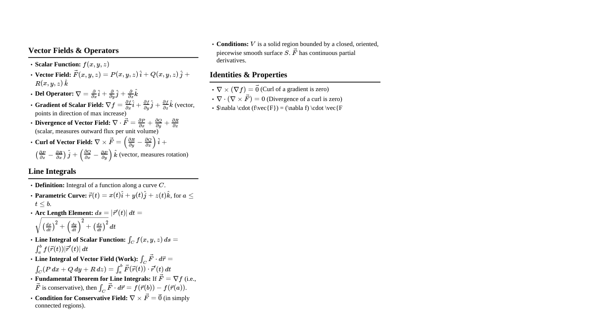
# VECTOR CALCULUS: LINE INTEGRALS – COMPLETE CONCEPTUAL GUIDE --- ### PART 1: MASTER OVERVIEW PAGE #### 1. Big Picture Introduction What is this chapter really about? This chapter, "Line Integrals," is fundamentally about extending the concept of integration from a one-dimensional interval on the real line to integration along a curve in multi-dimensional space. In elementary calculus, we integrate a function $f(x)$ over an interval $[a, b]$ to find the area under the curve or the accumulated change. Here, we generalize this idea: instead of integrating over a segment of the x-axis, we integrate over a path, or "line," in 2D or 3D space. This path can be straight or curved, open or closed. Why does it exist in mathematics? Line integrals exist because many physical phenomena are inherently path-dependent or involve quantities distributed along a curve. For instance, calculating the work done by a variable force along a curved trajectory, determining the mass of a wire with varying density, or finding the flow rate of a fluid along a particular path in a vector field—all these require integration over a curve. Standard Riemann integration is insufficient for these tasks because it lacks the geometric flexibility to account for the shape and orientation of the path. What problem was it created to solve? The primary problem line integrals were created to solve is the accurate summation of infinitesimally small quantities that vary along a given curve. Imagine a curve in space. At each point along this curve, we might have a different value for some scalar quantity (like temperature) or a different vector quantity (like a force). How do we sum up these values along the entire length of the curve, respecting its geometry? Line integrals provide the rigorous mathematical framework for this summation. They allow us to calculate total quantities that accumulate along a path, where both the quantity itself and the path's orientation contribute to the total. Real world motivation Consider the following scenarios: 1. **Work Done by a Force:** If you push a cart up a winding hill, the force you apply might change in magnitude and direction at every point, and the path itself is curved. The total work done cannot be found by simply multiplying force by distance; you need to sum the infinitesimal work done over each tiny segment of the path, where the force and displacement vectors are locally relevant. 2. **Mass of a Wire:** Imagine a thin wire bent into a complex shape, and its density varies along its length (e.g., thicker in some parts, thinner in others). To find the total mass, you must sum the infinitesimal masses along each segment of the wire, taking into account its varying density and geometry. 3. **Fluid Flow:** If you want to calculate how much fluid is flowing along a specific closed loop in a river (circulation), you need to sum the component of the fluid's velocity that is tangent to the loop at each point. Historical intuition The genesis of line integrals is deeply intertwined with the development of mechanics and electromagnetism in the 18th and 19th centuries. Physicists and mathematicians like Lagrange, Green, and Stokes grappled with problems involving forces, work, and fluid dynamics in complex geometries. They recognized that the standard calculus of single-variable integration was inadequate for these tasks. The concept evolved from summing infinitesimal contributions along a path, leading to the formalization of integrals over curves, which then paved the way for the powerful integral theorems (Green's, Stokes', Divergence Theorems) that unify vector calculus. The intuition was always about "summing up" effects along a specific trajectory, where the direction of movement along that trajectory was crucial. #### 2. Concept Map Structure ``` Chapter: Line Integrals ├── 1. Introduction to Line Integrals │ ├── 1.1. Motivation: Beyond Single-Variable Integration │ └── 1.2. Parametrization of Curves: The Foundation │ ├── 1.2.1. Vector-Valued Functions of a Single Parameter │ └── 1.2.2. Arc Length and Speed ├── 2. Line Integrals of Scalar Fields │ ├── 2.1. Definition: Integrating Scalar Functions along a Curve │ ├── 2.2. Geometric Interpretation: Area of a "Fence" │ ├── 2.3. Calculation: Reduction to Single-Variable Integral │ └── 2.4. Physical Applications: Mass of a Wire, Charge on a Curve ├── 3. Line Integrals of Vector Fields │ ├── 3.1. Definition: Integrating Vector Functions along a Curve │ ├── 3.2. Geometric Interpretation: Work Done, Circulation │ ├── 3.3. Calculation: Dot Product with Tangent Vector │ └── 3.4. Physical Applications: Work, Fluid Flow, Electromotive Force ├── 4. Properties of Line Integrals │ ├── 4.1. Orientation Dependence │ ├── 4.2. Additivity │ └── 4.3. Independence of Parametrization (for scalar fields) ├── 5. Fundamental Theorem for Line Integrals │ ├── 5.1. Conservative Vector Fields: Path Independence │ ├── 5.2. Potential Functions │ ├── 5.3. Connection to Gradient │ └── 5.4. Conditions for Conservatism (Curl Test) ├── 6. Applications and Advanced Concepts │ ├── 6.1. Green's Theorem (Introduction) │ ├── 6.2. Path Independence and Potential Energy │ └── 6.3. Flux across a Curve (2D) ``` #### 3. Logical Flow of Learning The chapter is structured to build understanding incrementally, moving from the most basic prerequisite to advanced applications. - **Topic 1 (Introduction to Line Integrals):** We begin by establishing *why* line integrals are necessary by highlighting the limitations of single-variable integration for path-dependent problems. The most crucial prerequisite for line integrals is the ability to describe curves mathematically. Hence, we immediately introduce **parametrization of curves** using vector-valued functions. Without a parametric representation, a line integral cannot be computed. We also touch upon arc length, which is intrinsically linked to integrating along a path. - **Topic 2 (Line Integrals of Scalar Fields):** Once curves are parametrized, we tackle the simpler case: integrating a scalar function. This is analogous to finding the "area under a curve" in 1D, but here it's the "area of a fence" over a curve. This concept is more straightforward as it only involves magnitude accumulation along the curve's length, setting the stage for the more complex vector field integrals. - **Topic 3 (Line Integrals of Vector Fields):** This is the core of the chapter. Building on the scalar case, we introduce the crucial concept of the dot product between the vector field and the infinitesimal tangent vector along the curve. This dot product captures the "alignment" between the field and the direction of movement, which is essential for understanding work, flow, and circulation. This naturally follows the scalar case as it adds the layer of directional interaction. - **Topic 4 (Properties of Line Integrals):** Having defined both types of line integrals, we then examine their fundamental properties. **Orientation dependence** is a critical distinction, especially for vector field integrals, and is a direct consequence of the dot product with the tangent vector. **Additivity** is a natural extension from standard integration. **Independence of parametrization** for scalar fields (and for some vector fields under specific conditions) reassures us that the result is a property of the curve and field, not our chosen description. - **Topic 5 (Fundamental Theorem for Line Integrals):** This is a profound conceptual leap. It connects line integrals of *certain* vector fields (conservative fields) directly to the values of a scalar potential function at the endpoints of the path. This is a direct generalization of the Fundamental Theorem of Calculus. This topic naturally follows the discussion of vector field integrals and their properties, as it introduces a condition under which path dependence disappears, simplifying calculations dramatically. The **curl test** naturally links back to the "curl" concept from the previous chapter. - **Topic 6 (Applications and Advanced Concepts):** Finally, we explore broader applications and introduce concepts that foreshadow future chapters (like Green's Theorem, which generalizes line integrals to area integrals). This demonstrates the power and utility of line integrals in various scientific and engineering contexts. What mental shift is required to understand this chapter The most significant mental shift is moving from thinking about "area under a curve" or "total change over an interval" to "summing quantities *along* a curve." This requires: 1. **Thinking parametrically:** Instead of $y=f(x)$, envision $\vec{r}(t) = \langle x(t), y(t), z(t) \rangle$. The curve is traced out over time or some other parameter. 2. **Infinitesimal displacement:** Understanding $d\vec{r}$ as a tiny vector tangent to the curve, giving both magnitude ($ds$) and direction. 3. **Directional interaction:** For vector fields, grasping that only the component of the field parallel to the path contributes to the integral, quantified by the dot product. This is a departure from scalar integration where all values contribute equally. 4. **Path dependence vs. independence:** Recognizing that the value of an integral can depend not just on the start and end points, but on the specific route taken between them, and discerning when this dependence vanishes. #### 4. Core Philosophy of the Chapter What deep idea connects everything? The core philosophy is the **quantification of accumulation along a path**. It's about how "things" (scalar values, vector effects) add up as one traverses a specific trajectory in space, and how the geometry of that trajectory and the orientation of the "things" relative to the trajectory profoundly influence the total accumulation. It's a testament to the power of calculus to model continuous processes over complex geometries. The deep idea is that *geometry matters* when summing quantities that vary spatially. What misconception students usually have? The most common misconception is treating a line integral as a simple definite integral $\int_a^b f(x) dx$. Students often forget: - **The curve matters:** The path of integration is not just the x-axis; it's a specific curve $C$. - **The differential element matters:** It's not just $dx$; it's $ds$ (arc length) for scalar fields or $d\vec{r}$ (displacement vector) for vector fields, which inherently incorporate the curve's geometry. - **Direction matters:** For vector fields, the relative orientation of the field and the path (via the dot product) is crucial. A force perpendicular to the path does no work. Another misconception is confusing line integrals of scalar fields with line integrals of vector fields. They look similar in notation but represent fundamentally different physical quantities and require different interpretations. What is the "soul" of this chapter? The "soul" of this chapter is the **precise measurement of interaction and accumulation over a continuous, curvilinear path**. It's about moving from static point-wise analysis to dynamic, path-dependent summation. It provides the mathematical language to describe how forces *do work* over a journey, how fields *circulate* around a loop, or how properties *distribute* along a physical object with shape. It is the bridge between the local behavior of fields and global, macroscopic effects, laying the groundwork for the fundamental integral theorems of vector calculus. It embodies the idea that "the whole is more than the sum of its parts" when those parts interact directionally along a path. --- ### PART 2: COMPLETE STRUCTURED THEORY NOTES #### 1. Introduction to Line Integrals ##### 1.1. Motivation: Beyond Single-Variable Integration **Definition:** Single-variable integration, $\int_a^b f(x) dx$, computes the signed area under the curve $y=f(x)$ from $x=a$ to $x=b$. It sums infinitesimal quantities $f(x)dx$ along a straight line segment of the x-axis. **Intuition:** Imagine a flat landscape. $\int_a^b f(x) dx$ tells you the area of a vertical slice of this landscape, where the base is a straight line segment on the ground. This is powerful for many problems where quantities vary along a single dimension. **Why it makes sense:** This form of integration works perfectly when the domain of integration is a simple interval on the real number line, and the function's variation is solely dependent on that single independent variable. **Logical Explanation:** The Riemann sum partitions the interval $[a, b]$ into small pieces $\Delta x_i$. For each piece, we approximate $f(x)$ as constant, $f(x_i^*)$, and sum $f(x_i^*)\Delta x_i$. Taking the limit as $\Delta x_i \to 0$ yields the integral. This assumes the path is always along the x-axis. **Geometric/Physical Interpretation:** * **Geometric:** Area under a curve. * **Physical:** Total displacement given velocity as a function of time, total charge accumulated along a line, total mass of a rod with varying density. **Real Life Example:** Calculating the total distance traveled by a car if its speed $v(t)$ is known over a time interval $[t_1, t_2]$. Here, distance $= \int_{t_1}^{t_2} v(t) dt$. **Common Mistakes:** Applying this 1D thinking to problems where the path is curved or where the quantity being summed interacts directionally with the path. **Connection to Previous Chapter:** Builds directly on the concept of definite integrals from single-variable calculus, highlighting its limitations and setting the stage for generalization. **Connection to Next Chapter:** Line integrals are the direct generalization, providing the necessary mathematical tool for describing path-dependent accumulation in higher dimensions. ##### 1.2. Parametrization of Curves: The Foundation **Definition:** A **parametrization** of a curve $C$ in $\mathbb{R}^2$ or $\mathbb{R}^3$ is a vector-valued function $\vec{r}(t) = \langle x(t), y(t) \rangle$ or $\vec{r}(t) = \langle x(t), y(t), z(t) \rangle$, where $t$ is a scalar parameter (often representing time) over an interval $[a, b]$. As $t$ varies from $a$ to $b$, the tip of the vector $\vec{r}(t)$ traces out the curve $C$. **Intuition:** Instead of describing a curve as $y=f(x)$ (which fails for vertical lines or self-intersecting curves), we describe it as a "journey." At each "time" $t$, you are at a specific position $(x(t), y(t), z(t))$. The parameter $t$ acts like a clock, guiding you along the path. **Why it makes sense:** Parametrization allows us to describe virtually any curve, regardless of whether it passes the vertical line test or can be described by a simple function of $x$ or $y$. It provides a consistent framework for describing the position, direction, and speed of movement along a curve. **Logical Explanation:** For each value of $t$ in the parameter interval, $\vec{r}(t)$ outputs a unique point in space. As $t$ smoothly changes, these points form a continuous curve. The functions $x(t)$, $y(t)$, and $z(t)$ must be continuous and differentiable for the curve to be smooth. **Step-by-step Derivation:** (No derivation for definition, but for related concepts like arc length) **Geometric/Physical Interpretation:** * **Geometric:** The path traced by a moving point. The parameter $t$ doesn't necessarily have to be time; it can be an angle, arc length, or any convenient variable. * **Physical:** The trajectory of a particle in motion, where $t$ is time, and $\vec{r}(t)$ is its position vector. **Real Life Example:** The path of a roller coaster, the flight path of an airplane, or the trajectory of a thrown ball can all be described parametrically. For instance, a circle of radius $R$ centered at the origin can be parametrized by $\vec{r}(t) = \langle R\cos t, R\sin t \rangle$ for $0 \le t \le 2\pi$. **Common Mistakes:** * Forgetting the parameter interval $[a, b]$. A parametrization is incomplete without specifying the range of $t$. * Confusing the parameter $t$ with a coordinate variable like $x$ or $y$. **Connection to Previous Chapter:** Builds on vector-valued functions and their derivatives from vector differentiation. The derivative $\vec{r}'(t)$ is the tangent vector to the curve. **Connection to Next Chapter:** Essential prerequisite for defining and calculating line integrals. Every line integral calculation begins with parametrizing the curve. ###### 1.2.1. Vector-Valued Functions of a Single Parameter **Definition:** A vector-valued function $\vec{r}(t)$ maps a single real number $t$ from its domain to a vector in $\mathbb{R}^n$ (typically $\mathbb{R}^2$ or $\mathbb{R}^3$). $\vec{r}(t) = x(t)\hat{i} + y(t)\hat{j}$ (for 2D) or $\vec{r}(t) = x(t)\hat{i} + y(t)\hat{j} + z(t)\hat{k}$ (for 3D). **Intuition:** Think of a continuously moving pointer (the vector $\vec{r}(t)$) whose tail is fixed at the origin. As $t$ changes, the tip of this pointer draws a curve in space. **Why it makes sense:** It provides a compact and powerful way to represent a curve, encapsulating all coordinate information in a single function. **Logical Explanation:** Each component function ($x(t), y(t), z(t)$) is a standard scalar function of $t$. The vector $\vec{r}(t)$ is formed by these components. **Geometric/Physical Interpretation:** The position vector of a particle at time $t$. ###### 1.2.2. Arc Length and Speed **Definition:** * The **velocity vector** is $\vec{v}(t) = \vec{r}'(t) = \langle x'(t), y'(t), z'(t) \rangle$. * The **speed** of the particle is the magnitude of the velocity vector: $|\vec{v}(t)| = |\vec{r}'(t)| = \sqrt{(x'(t))^2 + (y'(t))^2 + (z'(t))^2}$. * The **arc length** of a curve $C$ from $t=a$ to $t=b$ is given by $L = \int_a^b |\vec{r}'(t)| dt$. **Intuition:** Speed is how fast you're moving along the path at any instant. Arc length is the total distance traveled along the path. We sum up all the tiny distances traveled, $|\vec{r}'(t)|dt$. **Why it makes sense:** The infinitesimal displacement vector along the curve is $d\vec{r} = \vec{r}'(t)dt$. Its magnitude, $|d\vec{r}| = |\vec{r}'(t)|dt$, is the infinitesimal arc length, $ds$. Integrating $ds$ gives total arc length. **Logical Explanation:** This is a direct application of the Pythagorean theorem in the limit. For a tiny time interval $dt$, the particle moves $\Delta x = x'(t)dt$, $\Delta y = y'(t)dt$, $\Delta z = z'(t)dt$. The distance covered is $\sqrt{(\Delta x)^2 + (\Delta y)^2 + (\Delta z)^2} = \sqrt{(x'(t)dt)^2 + (y'(t)dt)^2 + (z'(t)dt)^2} = \sqrt{(x'(t))^2 + (y'(t))^2 + (z'(t))^2} dt = |\vec{r}'(t)|dt$. **Geometric/Physical Interpretation:** * **Geometric:** The length of a curved segment. * **Physical:** The distance an object travels along its trajectory. **Real Life Example:** If a space probe's trajectory is given by $\vec{r}(t)$, its speed at any moment is $|\vec{r}'(t)|$, and the total distance it travels over a mission segment is the arc length integral. **Common Mistakes:** Forgetting the square root in the speed/arc length formula. Confusing speed with velocity (speed is a scalar, velocity is a vector). **Connection to Previous Chapter:** Directly uses vector differentiation concepts ($\vec{r}'(t)$). **Connection to Next Chapter:** The infinitesimal arc length element $ds = |\vec{r}'(t)|dt$ is a crucial component in line integrals of scalar fields. #### 2. Line Integrals of Scalar Fields ##### 2.1. Definition: Integrating Scalar Functions along a Curve **Definition:** The line integral of a scalar function $f(x, y, z)$ along a smooth curve $C$ parametrized by $\vec{r}(t) = \langle x(t), y(t), z(t) \rangle$ for $a \le t \le b$ is given by: $$\int_C f(x, y, z) ds = \int_a^b f(x(t), y(t), z(t)) |\vec{r}'(t)| dt$$ where $ds = |\vec{r}'(t)| dt$ is the differential arc length element. **Intuition:** Imagine a thin, curved wire (the curve $C$) in space. At each point $(x,y,z)$ on the wire, there is a scalar value $f(x,y,z)$ associated with it (e.g., its linear mass density, or temperature). We want to find the total "amount" of this quantity along the entire wire. We do this by taking tiny segments of the wire, $ds$, multiplying by the value of $f$ at that segment, and summing them all up. **Why it makes sense:** This integral is a natural generalization of the definite integral $\int_a^b g(t) dt$. Here, the function $f$ is evaluated along the curve $C$, transforming $f(x,y,z)$ into $f(x(t),y(t),z(t))$, a function of $t$. The $ds$ element ensures that we are summing over the *actual length* of the curve, accounting for its curvature and not just its projection onto an axis. **Logical Explanation:** 1. **Parametrization:** The curve $C$ is described by $\vec{r}(t)$, which maps the 1D parameter interval $[a,b]$ to the curve in 3D space. 2. **Function evaluation:** The scalar function $f(x,y,z)$ is evaluated *along* the curve. This means we substitute $x(t), y(t), z(t)$ into $f$, making it a function of $t$: $f(\vec{r}(t))$. 3. **Differential arc length:** The infinitesimal length element $ds$ along the curve is given by $ds = |\vec{r}'(t)| dt$. This factor correctly scales the contribution of $f(\vec{r}(t))$ according to how fast the curve is being traced out (i.e., how "stretched" or "compressed" each $\Delta t$ interval becomes in terms of actual arc length). **Step-by-step Derivation (Riemann Sum approach):** 1. Divide the parameter interval $[a, b]$ into $n$ subintervals of width $\Delta t = (b-a)/n$. 2. This partitions the curve $C$ into $n$ small segments $C_k$. 3. Choose a sample point $\vec{r}(t_k^*)$ on each segment $C_k$. 4. The length of the $k$-th segment, $\Delta s_k$, can be approximated by $|\vec{r}'(t_k^*)| \Delta t$. 5. Form the Riemann sum: $\sum_{k=1}^n f(\vec{r}(t_k^*)) \Delta s_k = \sum_{k=1}^n f(x(t_k^*), y(t_k^*), z(t_k^*)) |\vec{r}'(t_k^*)| \Delta t$. 6. Taking the limit as $n \to \infty$ (and $\Delta t \to 0$) yields the definite integral: $$\int_a^b f(x(t), y(t), z(t)) |\vec{r}'(t)| dt$$ **Geometric/Physical Interpretation:** * **Geometric:** If $f(x,y,z) \ge 0$, the line integral $\int_C f(x,y,z) ds$ represents the area of a "fence" or "curtain" whose base is the curve $C$ and whose height at any point $(x,y,z)$ on $C$ is given by $f(x,y,z)$. * **Physical:** * If $f(x,y,z)$ is the linear mass density (mass per unit length) of a wire shaped like $C$, then $\int_C f(x,y,z) ds$ gives the total mass of the wire. * If $f(x,y,z)$ is the charge density along a curved filament, the integral gives the total charge. **Real Life Example:** Consider a thin, semicircular wire of radius $R$ in the $xy$-plane, with linear mass density $\rho(x,y) = kx^2$. To find its total mass: 1. Parametrize the semicircle: $\vec{r}(t) = \langle R\cos t, R\sin t \rangle$ for $0 \le t \le \pi$. 2. Find $\vec{r}'(t) = \langle -R\sin t, R\cos t \rangle$. 3. Find $|\vec{r}'(t)| = \sqrt{(-R\sin t)^2 + (R\cos t)^2} = \sqrt{R^2\sin^2 t + R^2\cos^2 t} = \sqrt{R^2} = R$. 4. Evaluate $\rho$ along the curve: $\rho(x(t), y(t)) = k(R\cos t)^2 = kR^2\cos^2 t$. 5. Set up the integral: $\int_C \rho(x,y) ds = \int_0^\pi (kR^2\cos^2 t) (R) dt = kR^3 \int_0^\pi \cos^2 t dt$. 6. Use the identity $\cos^2 t = \frac{1+\cos(2t)}{2}$: $kR^3 \int_0^\pi \frac{1+\cos(2t)}{2} dt = \frac{kR^3}{2} \left[ t + \frac{1}{2}\sin(2t) \right]_0^\pi$ $= \frac{kR^3}{2} [(\pi + 0) - (0 + 0)] = \frac{\pi kR^3}{2}$. This is the total mass. **Common Mistakes:** * Forgetting to convert $f(x,y,z)$ into $f(x(t),y(t),z(t))$. * Forgetting the $|\vec{r}'(t)|$ factor in the integral, effectively integrating with respect to $t$ instead of arc length $s$. * Incorrectly calculating $|\vec{r}'(t)|$. **Connection to Previous Chapter:** Relies on the ability to parametrize curves and calculate their arc length. **Connection to Next Chapter:** Serves as a simpler conceptual step before tackling line integrals of vector fields, where directional interaction becomes paramount. #### 3. Line Integrals of Vector Fields ##### 3.1. Definition: Integrating Vector Functions along a Curve **Definition:** The line integral of a vector field $\vec{F}(x, y, z) = P(x,y,z)\hat{i} + Q(x,y,z)\hat{j} + R(x,y,z)\hat{k}$ along a smooth curve $C$ parametrized by $\vec{r}(t) = \langle x(t), y(t), z(t) \rangle$ for $a \le t \le b$ is given by: $$\int_C \vec{F} \cdot d\vec{r} = \int_a^b \vec{F}(x(t), y(t), z(t)) \cdot \vec{r}'(t) dt$$ where $d\vec{r} = \vec{r}'(t) dt$ is the differential displacement vector. Alternatively, in component form: $$\int_C P dx + Q dy + R dz = \int_a^b \left(P(x(t),y(t),z(t))x'(t) + Q(x(t),y(t),z(t))y'(t) + R(x(t),y(t),z(t))z'(t)\right) dt$$ **Intuition:** Imagine you are walking along a path $C$ in a force field $\vec{F}$ (like gravity or wind). At each tiny step you take, $d\vec{r}$, the force $\vec{F}$ might be pushing or pulling you. The work done by the force over that tiny step is $\vec{F} \cdot d\vec{r}$ (force component in direction of motion times distance). The line integral sums up all these tiny bits of work along the entire path. If the force helps you, it's positive work; if it hinders you, it's negative. **Why it makes sense:** This integral quantifies the *net effect* of a vector field along a path, specifically how much the field tends to *align* with the direction of movement. The dot product $\vec{F} \cdot d\vec{r}$ is crucial because it isolates the component of the vector field that is parallel to the infinitesimal displacement. Only this parallel component contributes to the "flow" or "work" along the path. **Logical Explanation:** 1. **Parametrization:** As before, $\vec{r}(t)$ describes the curve $C$. 2. **Vector Field Evaluation:** The vector field $\vec{F}$ is evaluated at points along the curve, $\vec{F}(\vec{r}(t))$. This transforms $\vec{F}$ into a vector function of $t$. 3. **Differential Displacement:** The infinitesimal displacement vector $d\vec{r} = \vec{r}'(t)dt$ points in the tangent direction of the curve and has a magnitude of $ds$. 4. **Dot Product:** The core of the line integral of a vector field is the dot product $\vec{F}(\vec{r}(t)) \cdot \vec{r}'(t)$. This calculates the scalar projection of the force (or field) onto the direction of motion at each point. This is a scalar function of $t$. 5. **Integration:** The integral then sums these scalar contributions over the parameter interval $[a,b]$, yielding a single scalar value representing the total accumulation (e.g., total work). **Step-by-step Derivation (Riemann Sum approach):** 1. Divide the parameter interval $[a, b]$ into $n$ subintervals of width $\Delta t = (b-a)/n$. 2. This partitions the curve $C$ into $n$ small segments. 3. Choose a sample point $\vec{r}(t_k^*)$ on each segment $C_k$. 4. The infinitesimal displacement vector for the $k$-th segment is approximated by $\Delta \vec{r}_k = \vec{r}'(t_k^*) \Delta t$. This vector points approximately along the segment $C_k$. 5. Evaluate the vector field at the sample point: $\vec{F}(\vec{r}(t_k^*))$. 6. The contribution of the field over this segment is approximately $\vec{F}(\vec{r}(t_k^*)) \cdot \Delta \vec{r}_k = \vec{F}(\vec{r}(t_k^*)) \cdot \vec{r}'(t_k^*) \Delta t$. 7. Form the Riemann sum: $\sum_{k=1}^n \vec{F}(\vec{r}(t_k^*)) \cdot \vec{r}'(t_k^*) \Delta t$. 8. Taking the limit as $n \to \infty$ yields the definite integral: $$\int_a^b \vec{F}(x(t), y(t), z(t)) \cdot \vec{r}'(t) dt$$ **Geometric/Physical Interpretation:** * **Work Done:** If $\vec{F}$ is a force field, $\int_C \vec{F} \cdot d\vec{r}$ represents the total work done by the force field in moving a particle along the curve $C$. If the integral is positive, the field helps the movement; if negative, it opposes it. * **Circulation:** If $C$ is a closed curve, the line integral $\oint_C \vec{F} \cdot d\vec{r}$ (the circle on the integral sign denotes a closed path) represents the **circulation** of the vector field around the curve. This is a measure of the field's tendency to rotate fluid or to induce a voltage in a loop. * **Flow/Flux (tangential component):** The integral measures the total "flow" of the vector field *along* the curve. **Real Life Example:** Consider a particle moving along a parabolic path $C$ given by $\vec{r}(t) = \langle t, t^2 \rangle$ from $(0,0)$ to $(1,1)$ in a force field $\vec{F}(x,y) = \langle -y, x \rangle$. Find the work done. 1. Parameter interval: $t$ goes from $0$ to $1$. 2. Derivative of parametrization: $\vec{r}'(t) = \langle 1, 2t \rangle$. 3. Evaluate $\vec{F}$ along the curve: $\vec{F}(x(t), y(t)) = \vec{F}(t, t^2) = \langle -t^2, t \rangle$. 4. Compute the dot product: $\vec{F}(\vec{r}(t)) \cdot \vec{r}'(t) = \langle -t^2, t \rangle \cdot \langle 1, 2t \rangle = (-t^2)(1) + (t)(2t) = -t^2 + 2t^2 = t^2$. 5. Set up and evaluate the integral: Work $= \int_C \vec{F} \cdot d\vec{r} = \int_0^1 t^2 dt = \left[ \frac{t^3}{3} \right]_0^1 = \frac{1}{3} - 0 = \frac{1}{3}$. The work done is $1/3$ units. **Common Mistakes:** * Confusing $\int_C f ds$ with $\int_C \vec{F} \cdot d\vec{r}$. The former uses $f(\vec{r}(t))|\vec{r}'(t)|dt$, the latter uses $\vec{F}(\vec{r}(t)) \cdot \vec{r}'(t)dt$. One involves scalar magnitude, the other a directional interaction. * Forgetting the dot product. This is critical for vector field line integrals. * Incorrectly substituting $x(t), y(t), z(t)$ into the vector field $\vec{F}$. * Errors in differentiating $\vec{r}(t)$ or performing the dot product. **Connection to Previous Chapter:** Builds heavily on parametrization of curves and understanding of vector fields, dot products, and derivatives of vector functions. **Connection to Next Chapter:** Crucial for understanding Green's Theorem, Stokes' Theorem, and the Fundamental Theorem for Line Integrals, which simplify calculations for specific types of vector fields. #### 4. Properties of Line Integrals ##### 4.1. Orientation Dependence **Definition:** The **orientation** of a curve $C$ refers to the direction in which it is traversed. If $C$ is traversed from point A to point B, then $-C$ denotes the same curve traversed from B to A. **Intuition:** Imagine walking up a hill. The work done by gravity is negative. If you walk down the same path, the work done by gravity is positive. The force of gravity hasn't changed, but your direction of movement has. **Why it makes sense:** * For **scalar field line integrals** ($\int_C f ds$): The integral is *independent* of the orientation. The differential arc length $ds$ is a scalar magnitude, always positive. $ds = |\vec{r}'(t)|dt = |-\vec{r}'(t)|dt$. So, $\int_C f ds = \int_{-C} f ds$. The total mass of a wire doesn't depend on which end you start measuring from. * For **vector field line integrals** ($\int_C \vec{F} \cdot d\vec{r}$): The integral *depends* on the orientation. The differential displacement vector $d\vec{r} = \vec{r}'(t)dt$ changes sign if the parametrization is reversed (e.g., if $\vec{r}_{rev}(t) = \vec{r}(a+b-t)$, then $\vec{r}_{rev}'(t) = -\vec{r}'(a+b-t)$). Therefore, $\int_{-C} \vec{F} \cdot d\vec{r} = -\int_C \vec{F} \cdot d\vec{r}$. The work done in going up a hill is the negative of the work done in going down the same hill. **Logical Explanation:** The dot product $\vec{F} \cdot d\vec{r}$ involves the direction of $d\vec{r}$. If the direction of $d\vec{r}$ is reversed, the dot product changes sign (since $\vec{A} \cdot (-\vec{B}) = -(\vec{A} \cdot \vec{B})$). This sign change propagates through the integral. For scalar integrals, $ds$ is always positive, so there's no sign change. **Geometric/Physical Interpretation:** * **Work:** If you walk against a headwind, the wind does negative work. If you walk with a tailwind, it does positive work. The same wind field, but opposite directions of travel, yield opposite work values. * **Circulation:** If the circulation of a fluid around a loop is clockwise, reversing the path to counter-clockwise will give the negative circulation. **Common Mistakes:** Assuming that all line integrals are orientation-dependent. Incorrectly applying the sign change for scalar line integrals. ##### 4.2. Additivity **Definition:** If a curve $C$ is composed of several smooth sub-curves $C_1, C_2, \ldots, C_n$ joined end-to-end (i.e., $C = C_1 \cup C_2 \cup \ldots \cup C_n$), then the line integral over $C$ is the sum of the line integrals over each sub-curve. $$\int_C f ds = \int_{C_1} f ds + \int_{C_2} f ds + \ldots + \int_{C_n} f ds$$ $$\int_C \vec{F} \cdot d\vec{r} = \int_{C_1} \vec{F} \cdot d\vec{r} + \int_{C_2} \vec{F} \cdot d\vec{r} + \ldots + \int_{C_n} \vec{F} \cdot d\vec{r}$$ **Intuition:** If you measure the total mass of a long, bent wire, you can break it into smaller segments, find the mass of each segment, and add them up. The total work done along a complicated path is the sum of the work done along each segment of that path. **Why it makes sense:** This property directly follows from the additivity of definite integrals. The integral is a summation process, and summing parts of a whole yields the total sum. **Logical Explanation:** The parameter interval $[a,b]$ for $C$ can be broken into subintervals corresponding to $C_1, \ldots, C_n$. The integral over $[a,b]$ is the sum of integrals over these subintervals. **Real Life Example:** Calculating the work done by a force field along a square path. You can calculate the work along each of the four sides and sum them up. **Common Mistakes:** Forgetting to handle the parametrization of each sub-curve separately, ensuring that the starting point of $C_{i+1}$ matches the endpoint of $C_i$. ##### 4.3. Independence of Parametrization (for scalar fields) **Definition:** For line integrals of scalar fields, the value of $\int_C f ds$ is independent of the particular parametrization $\vec{r}(t)$ used to describe the curve $C$, as long as the parametrization traces the curve in the same direction. **Intuition:** If you're measuring the total mass of a wire, it shouldn't matter if you describe your journey along the wire as taking 10 seconds or 10 minutes, or if you walk quickly or slowly. As long as you cover the entire wire, the total mass remains the same. **Why it makes sense:** The differential arc length $ds = |\vec{r}'(t)|dt$ acts as a scaling factor that normalizes the integral with respect to the speed of parametrization. If you parametrize the curve faster (larger $|\vec{r}'(t)|$), the $dt$ interval becomes smaller for a given $ds$. The product $|\vec{r}'(t)|dt$ ensures that the actual length element $ds$ is always used. **Logical Explanation:** Let $C$ be parametrized by $\vec{r}_1(t)$ for $t \in [a,b]$ and by $\vec{r}_2(u)$ for $u \in [c,d]$. If $\vec{r}_1(t)$ and $\vec{r}_2(u)$ trace the same curve $C$ in the same direction, then there exists a strictly increasing change of parameter function $t=g(u)$ such that $\vec{r}_1(g(u)) = \vec{r}_2(u)$. Using the chain rule, $\frac{d\vec{r}_1}{du} = \frac{d\vec{r}_1}{dt}\frac{dt}{du}$. Then $\int_c^d f(\vec{r}_2(u)) |\vec{r}_2'(u)| du = \int_c^d f(\vec{r}_1(g(u))) |\vec{r}_1'(g(u))| \left|\frac{dg}{du}\right| du$. Since $g(u)$ is strictly increasing, $\frac{dg}{du} > 0$, so $|\frac{dg}{du}| = \frac{dg}{du}$. Let $t=g(u)$, $dt=\frac{dg}{du}du$. The integral becomes $\int_{g(c)}^{g(d)} f(\vec{r}_1(t)) |\vec{r}_1'(t)| dt = \int_a^b f(\vec{r}_1(t)) |\vec{r}_1'(t)| dt$. This confirms independence from parametrization for scalar line integrals. *Note: For vector field line integrals, this is also true if the orientation is preserved.* **Common Mistakes:** Confusing independence of parametrization with independence of path (which is a much stronger condition for vector fields). **Connection to Previous Chapter:** Reinforces the understanding of how parameter changes affect derivatives and integrals. **Connection to Next Chapter:** Sets the stage for understanding path independence in the context of conservative vector fields, where the integral's value depends only on endpoints, not the specific path. #### 5. Fundamental Theorem for Line Integrals ##### 5.1. Conservative Vector Fields: Path Independence **Definition:** A vector field $\vec{F}$ is called **conservative** if the line integral $\int_C \vec{F} \cdot d\vec{r}$ is **path independent**. This means that for any two points $A$ and $B$ in the domain of $\vec{F}$, the value of the line integral from $A$ to $B$ depends only on $A$ and $B$, and not on the particular path $C$ taken between them. An equivalent condition is that $\oint_C \vec{F} \cdot d\vec{r} = 0$ for every closed path $C$ in the domain of $\vec{F}$. **Intuition:** Imagine a gravitational field. If you lift an object from the floor to a shelf, the work done against gravity is the same regardless of whether you lift it straight up, or move it in a zigzag pattern, or even take it for a walk around the room before placing it on the shelf. The work done only depends on the change in elevation (start and end points). Such a field is conservative. A non-conservative field (like friction) would yield different work values for different paths. **Why it makes sense:** Path independence implies that there's no "net work" done if you return to your starting point. This suggests that the field is associated with a form of potential energy, where changes in potential energy depend only on the initial and final states. **Logical Explanation:** If the work done is independent of path, then traversing a path from A to B and then returning from B to A along a different path forms a closed loop. If the work is path independent, then $\int_A^B \vec{F} \cdot d\vec{r}$ (path 1) $= \int_A^B \vec{F} \cdot d\vec{r}$ (path 2). This means $\int_A^B \vec{F} \cdot d\vec{r}$ (path 1) - $\int_A^B \vec{F} \cdot d\vec{r}$ (path 2) $= 0$. Since $\int_A^B \vec{F} \cdot d\vec{r}$ (path 2) $= -\int_B^A \vec{F} \cdot d\vec{r}$ (path 2), we get $\int_A^B \vec{F} \cdot d\vec{r}$ (path 1) $+ \int_B^A \vec{F} \cdot d\vec{r}$ (path 2) $= 0$, which is the integral over the closed loop. **Geometric/Physical Interpretation:** * **Work/Energy:** Conservative forces are those for which work done is path independent. This implies the existence of a potential energy function. * **Physical fields:** Gravitational fields, electrostatic fields (in static cases) are conservative. Frictional forces, magnetic forces (in some contexts), or time-varying electric fields are generally non-conservative. **Common Mistakes:** Assuming all vector fields are conservative. Not understanding the equivalence between path independence and zero integral over closed loops. ##### 5.2. Potential Functions **Definition:** If a vector field $\vec{F}$ is conservative, then there exists a scalar function $\phi(x, y, z)$, called a **potential function** (or scalar potential), such that $\vec{F} = \nabla\phi$. The line integral of a conservative vector field $\vec{F}$ from point $A$ to point $B$ can then be calculated simply as: $$\int_C \vec{F} \cdot d\vec{r} = \phi(B) - \phi(A)$$ This is the **Fundamental Theorem for Line Integrals**. **Intuition:** Just as the definite integral of a derivative $f'(x)$ is $f(b)-f(a)$, the line integral of a gradient field $\nabla\phi$ is simply the difference in the potential function $\phi$ at the endpoints. The integral "undoes" the gradient, leaving only the change in the potential. **Why it makes sense:** If $\vec{F} = \nabla\phi$, then $d\phi = \frac{\partial\phi}{\partial x}dx + \frac{\partial\phi}{\partial y}dy + \frac{\partial\phi}{\partial z}dz = \nabla\phi \cdot d\vec{r} = \vec{F} \cdot d\vec{r}$. So, $\int_C \vec{F} \cdot d\vec{r} = \int_C d\phi$. This is a total differential. Integrating a total differential along a path simply gives the total change in the function from the start to the end. **Logical Explanation (Step-by-step Derivation):** Let $C$ be parametrized by $\vec{r}(t) = \langle x(t), y(t), z(t) \rangle$ for $a \le t \le b$, with $A = \vec{r}(a)$ and $B = \vec{r}(b)$. If $\vec{F} = \nabla\phi$, then: $$\int_C \vec{F} \cdot d\vec{r} = \int_a^b \vec{F}(\vec{r}(t)) \cdot \vec{r}'(t) dt$$ Substitute $\vec{F} = \nabla\phi$: $$= \int_a^b \nabla\phi(\vec{r}(t)) \cdot \vec{r}'(t) dt$$ By the chain rule for multivariable functions, the integrand is precisely the total derivative of $\phi$ with respect to $t$ along the curve: $$\frac{d}{dt}\phi(x(t), y(t), z(t)) = \frac{\partial\phi}{\partial x}\frac{dx}{dt} + \frac{\partial\phi}{\partial y}\frac{dy}{dt} + \frac{\partial\phi}{\partial z}\frac{dz}{dt} = \nabla\phi(\vec{r}(t)) \cdot \vec{r}'(t)$$ So, the integral becomes: $$= \int_a^b \frac{d}{dt}\phi(\vec{r}(t)) dt$$ By the Fundamental Theorem of Calculus: $$= \phi(\vec{r}(b)) - \phi(\vec{r}(a)) = \phi(B) - \phi(A)$$ This proves that if $\vec{F}$ is the gradient of a scalar function, its line integral depends only on the endpoints. **Geometric/Physical Interpretation:** * **Potential Energy:** In physics, a conservative force $\vec{F}$ is often expressed as the negative gradient of a potential energy function $U$: $\vec{F} = -\nabla U$. Then the work done by the force is $W = \int_C \vec{F} \cdot d\vec{r} = \int_C -\nabla U \cdot d\vec{r} = - (U(B) - U(A)) = U(A) - U(B)$. This means the work done by a conservative force equals the decrease in potential energy. * **Electric Potential:** In electrostatics, the electric field $\vec{E}$ is conservative and given by $\vec{E} = -\nabla V$, where $V$ is the electric potential. The voltage difference between two points is $V_B - V_A = -\int_A^B \vec{E} \cdot d\vec{r}$. **Real Life Example:** Calculating the work done by gravity. Gravity is a conservative force. For an object of mass $m$ near the Earth's surface, $\vec{F}_g = \langle 0, 0, -mg \rangle$. The gravitational potential function is $\phi(x,y,z) = -mgz$ (since $\nabla(-mgz) = \langle 0, 0, -mg \rangle = \vec{F}_g$). If an object moves from $A=(x_1,y_1,z_1)$ to $B=(x_2,y_2,z_2)$, the work done by gravity is $\phi(B) - \phi(A) = -mgz_2 - (-mgz_1) = mg(z_1 - z_2)$. This is the familiar $mg\Delta h$ formula. **Common Mistakes:** * Applying the Fundamental Theorem for Line Integrals to non-conservative fields. * Incorrectly finding the potential function $\phi$. ##### 5.3. Connection to Gradient **Definition:** A vector field $\vec{F}$ is conservative if and only if it is the gradient of some scalar potential function $\phi$. That is, $\vec{F}$ is conservative $\iff \vec{F} = \nabla\phi$. **Intuition:** The gradient always points in the direction of maximum increase of a scalar function. A field that is the gradient of a scalar function is inherently "smooth" and "non-rotational" in a way that allows for path independence. It's like navigating a landscape where the path to a certain altitude doesn't matter, only the starting and ending altitudes. **Why it makes sense:** If $\vec{F} = \nabla\phi$, then $\int_C \vec{F} \cdot d\vec{r} = \int_C \nabla\phi \cdot d\vec{r} = \phi(B) - \phi(A)$, which is path independent. Conversely, if the integral is path independent, it can be defined as $\phi(x,y,z) = \int_{(x_0,y_0,z_0)}^{(x,y,z)} \vec{F} \cdot d\vec{r}$, and then one can show that $\nabla\phi = \vec{F}$. **Logical Explanation:** This is the heart of the Fundamental Theorem. The gradient operation is the "antidifferentiation" for line integrals in conservative fields. **Connection to Previous Chapter:** Directly links the concept of conservative fields to the gradient operator introduced earlier. ##### 5.4. Conditions for Conservatism (Curl Test) **Definition:** For a vector field $\vec{F} = P\hat{i} + Q\hat{j} + R\hat{k}$ defined on a simply connected domain $D$ (meaning it has no "holes" and is in one piece): $\vec{F}$ is conservative $\iff \nabla \times \vec{F} = \vec{0}$ (i.e., $\vec{F}$ is irrotational). In component form, this means: $$\frac{\partial R}{\partial y} = \frac{\partial Q}{\partial z}$$ $$\frac{\partial P}{\partial z} = \frac{\partial R}{\partial x}$$ $$\frac{\partial Q}{\partial x} = \frac{\partial P}{\partial y}$$ **Intuition:** If a field has "swirl" or "rotation" (non-zero curl), then you can always find a closed loop around which there will be net work done. This means it cannot be path independent. Conversely, if there's no local swirl (zero curl), then the field can be thought of as flowing "straight" from higher potential to lower potential, leading to path independence. Think of a fluid: if it's swirling, you can put a paddle wheel in it and get it to turn, doing work. If it's irrotational, no paddle wheel will spin, and no work can be done around a closed loop. **Why it makes sense:** We previously proved the identity $\nabla \times (\nabla\phi) = \vec{0}$. If $\vec{F}$ is conservative, then $\vec{F} = \nabla\phi$ for some scalar potential $\phi$. Therefore, $\nabla \times \vec{F} = \nabla \times (\nabla\phi) = \vec{0}$. This shows that conservative fields *must* be irrotational. The converse (if $\nabla \times \vec{F} = \vec{0}$, then $\vec{F}$ is conservative) is true provided the domain $D$ is simply connected. The "simply connected" condition is important because a field with zero curl in a domain with a hole might still not be conservative (e.g., the field $\vec{F} = \langle -y/(x^2+y^2), x/(x^2+y^2) \rangle$ has zero curl everywhere except at the origin, but its line integral around a circle enclosing the origin is non-zero). **Logical Explanation:** The curl measures the infinitesimal rotation of a field. If there's no rotation anywhere, then there's no "energy loss" or "gain" by going around a loop. Thus, the total energy change (integral) only depends on the start and end. **Geometric/Physical Interpretation:** * **Irrotational Flow:** In fluid dynamics, a fluid flow field with zero curl is called an irrotational flow. * **Conservative Forces:** The curl test is a practical way to check if a force field is conservative, which then allows for the use of potential energy concepts. **Real Life Example:** Testing if $\vec{F}(x,y) = \langle 2xy, x^2 \rangle$ is conservative. Here $P=2xy$ and $Q=x^2$. Check if $\frac{\partial Q}{\partial x} = \frac{\partial P}{\partial y}$: $\frac{\partial Q}{\partial x} = \frac{\partial}{\partial x}(x^2) = 2x$. $\frac{\partial P}{\partial y} = \frac{\partial}{\partial y}(2xy) = 2x$. Since $\frac{\partial Q}{\partial x} = \frac{\partial P}{\partial y}$, the field is conservative (in $\mathbb{R}^2$, which is simply connected). We can then find a potential function $\phi$ such that $\nabla\phi = \vec{F}$. $\frac{\partial\phi}{\partial x} = 2xy \implies \phi(x,y) = x^2y + g(y)$. $\frac{\partial\phi}{\partial y} = x^2 + g'(y)$. Comparing this to $Q=x^2$, we get $x^2 + g'(y) = x^2 \implies g'(y) = 0 \implies g(y) = C$. So, $\phi(x,y) = x^2y + C$ is a potential function. **Common Mistakes:** * Forgetting the "simply connected domain" condition. * Incorrectly calculating partial derivatives for the curl components. * Confusing the conditions for 2D (only one curl component to check) with 3D (all three components). **Connection to Previous Chapter:** Directly uses the curl operator from the previous chapter. **Connection to Next Chapter:** This theorem is a special case of Green's Theorem (in 2D) and Stokes' Theorem (in 3D), which generalize the relationship between line integrals and derivatives of fields. #### 6. Applications and Advanced Concepts ##### 6.1. Green's Theorem (Introduction) **Definition:** Green's Theorem relates a line integral around a simple, closed, positively oriented curve $C$ in the plane to a double integral over the region $D$ bounded by $C$. $$\oint_C P dx + Q dy = \iint_D \left(\frac{\partial Q}{\partial x} - \frac{\partial P}{\partial y}\right) dA$$ **Intuition:** It's a 2D version of the Fundamental Theorem of Calculus. Instead of relating an integral to values at endpoints, it relates an integral over a boundary curve to an integral over the interior region. The term $(\frac{\partial Q}{\partial x} - \frac{\partial P}{\partial y})$ is the $z$-component of $\nabla \times \vec{F}$ for $\vec{F}=\langle P,Q \rangle$. So, it connects the "circulation" around the boundary to the "sum of infinitesimal rotations" within the region. **Why it makes sense:** It provides an alternative way to compute line integrals, often simplifying complex calculations by converting them to area integrals, or vice versa. It also formalizes the connection between a field's local rotational properties (curl) and its global circulation around a loop. **Logical Explanation:** The theorem essentially states that the total "swirl" of a vector field within a region is equal to the "flow" of the field along the boundary of that region. **Connection to Next Chapter:** Green's Theorem is a special case of Stokes' Theorem, which generalizes this idea to 3D surfaces and their boundary curves. ##### 6.2. Path Independence and Potential Energy **Definition:** For a conservative force field $\vec{F}$, the work done $W = \int_C \vec{F} \cdot d\vec{r}$ is path independent. This allows us to define a potential energy function $U$ such that $W = -\Delta U = U(A) - U(B)$. **Intuition:** This is the cornerstone of energy conservation in mechanics. If forces are conservative, mechanical energy (kinetic + potential) is conserved. It means we can associate a "stored energy" with a position in space. **Why it makes sense:** If work depends only on initial and final positions, then for a closed loop, the work done is zero. This means no energy is gained or lost by the system, consistent with energy conservation. **Connection to Physics:** Directly relates to the conservation of mechanical energy in physics. ##### 6.3. Flux across a Curve (2D) **Definition:** The **flux** of a 2D vector field $\vec{F} = \langle P, Q \rangle$ across a curve $C$ is the line integral of the normal component of $\vec{F}$ across $C$. It measures the rate at which the field "flows" across the curve. If $\vec{r}(t) = \langle x(t), y(t) \rangle$, the outward unit normal vector is often given by $\vec{n} = \langle y'(t), -x'(t) \rangle / |\vec{r}'(t)|$. Then the flux integral is $\int_C \vec{F} \cdot \vec{n} ds = \int_a^b \vec{F}(\vec{r}(t)) \cdot \langle y'(t), -x'(t) \rangle dt = \int_C P dy - Q dx$. **Intuition:** Imagine a river. If you place a small gate (a curve) in the river, the flux measures how much water flows *through* that gate perpendicular to it. It's about how much "stuff" is crossing the boundary, not flowing along it. **Why it makes sense:** The normal vector $\vec{n}$ ensures that only the component of the field perpendicular to the curve contributes to the flux. **Connection to Next Chapter:** This concept is generalized to surface integrals for flux across 3D surfaces and is central to the Divergence Theorem. --- ### PART 3: FORMULA SHEET #### A. Fundamental Definitions 1. **Parametrization of a Curve $C$ (3D):** * $\vec{r}(t) = x(t)\hat{i} + y(t)\hat{j} + z(t)\hat{k}$, for $a \le t \le b$. * **What it represents:** The position vector of a point on the curve at parameter $t$. * **When to use it:** To describe any curve in space, especially when $y=f(x)$ form is insufficient or inconvenient. * **Why it works:** Provides a systematic way to map a 1D interval to a multi-dimensional curve. * **Hidden assumptions:** $x(t), y(t), z(t)$ are continuous. 2. **Differential Arc Length Element ($ds$):** * $ds = |\vec{r}'(t)| dt = \sqrt{(x'(t))^2 + (y'(t))^2 + (z'(t))^2} dt$. * **What it represents:** An infinitesimally small length segment along the curve $C$. * **When to use it:** In line integrals of scalar fields, and for calculating total arc length. * **Why it works:** It's the magnitude of the infinitesimal displacement vector $d\vec{r}$, correctly accounting for curve geometry. * **Hidden assumptions:** $\vec{r}(t)$ is differentiable. 3. **Differential Displacement Vector ($d\vec{r}$):** * $d\vec{r} = \vec{r}'(t) dt = \langle x'(t), y'(t), z'(t) \rangle dt$. * **What it represents:** An infinitesimally small vector tangent to the curve $C$, pointing in the direction of increasing $t$. * **When to use it:** In line integrals of vector fields. * **Why it works:** It's the velocity vector scaled by $dt$, representing the direction and magnitude of an infinitesimal step along the curve. * **Hidden assumptions:** $\vec{r}(t)$ is differentiable. #### B. Core Identities 1. **Line Integral of a Scalar Field $f$ along $C$:** * $\int_C f(x, y, z) ds = \int_a^b f(x(t), y(t), z(t)) |\vec{r}'(t)| dt$. * **What it represents:** The total accumulation of a scalar quantity along a curve. * **When to use it:** To find mass of a wire, total charge, area of a fence, etc. * **Why it works:** Sums $f \cdot ds$ over the path, where $ds$ correctly measures length. * **Hidden assumptions:** $f$ is continuous on $C$, $C$ is smooth. 2. **Line Integral of a Vector Field $\vec{F}$ along $C$ (Work Integral):** * $\int_C \vec{F} \cdot d\vec{r} = \int_a^b \vec{F}(x(t), y(t), z(t)) \cdot \vec{r}'(t) dt$. * **What it represents:** The total work done by a force field, or total circulation of a vector field, along a curve. * **When to use it:** To find work done by a force, fluid circulation, voltage induced. * **Why it works:** Sums $\vec{F} \cdot d\vec{r}$ over the path, capturing the directional interaction. * **Hidden assumptions:** $\vec{F}$ is continuous on $C$, $C$ is smooth. #### C. Derived Results 1. **Fundamental Theorem for Line Integrals:** * If $\vec{F}$ is a conservative vector field (i.e., $\vec{F} = \nabla\phi$ for some scalar potential $\phi$), and $C$ is a path from point $A$ to point $B$, then $\int_C \vec{F} \cdot d\vec{r} = \phi(B) - \phi(A)$. * **What it represents:** The total change in potential function along the path. * **When to use it:** When $\vec{F}$ is known to be conservative, this simplifies line integral calculation by avoiding parametrization. * **Why it works:** The line integral of a gradient field is a total differential, which integrates to the difference in the potential function at the endpoints. * **Hidden assumptions:** $\vec{F}$ is conservative and defined on a domain where $\phi$ exists; $\phi$ is continuously differentiable. 2. **Condition for Conservatism (Curl Test) in 3D:** * If $\vec{F} = P\hat{i} + Q\hat{j} + R\hat{k}$ is defined on a simply connected domain $D$, then $\vec{F}$ is conservative if and only if $\nabla \times \vec{F} = \vec{0}$. * This implies: $\frac{\partial R}{\partial y} = \frac{\partial Q}{\partial z}$, $\frac{\partial P}{\partial z} = \frac{\partial R}{\partial x}$, $\frac{\partial Q}{\partial x} = \frac{\partial P}{\partial y}$. * **What it represents:** A test to determine if a given vector field is conservative. * **When to use it:** Before attempting to find a potential function or apply the Fundamental Theorem for Line Integrals. * **Why it works:** Conservative fields are precisely those that are irrotational. * **Hidden assumptions:** $\vec{F}$ has continuous partial derivatives; the domain is simply connected. 3. **Condition for Conservatism (Curl Test) in 2D:** * If $\vec{F} = P\hat{i} + Q\hat{j}$ is defined on a simply connected domain $D$, then $\vec{F}$ is conservative if and only if $\frac{\partial Q}{\partial x} = \frac{\partial P}{\partial y}$. * **What it represents:** A simplified test for 2D conservative fields. * **When to use it:** For 2D vector fields. * **Why it works:** It's the $z$-component of $\nabla \times \vec{F} = \vec{0}$ extended to 2D. * **Hidden assumptions:** $\vec{F}$ has continuous partial derivatives; the domain is simply connected. #### D. Special Cases 1. **Line Integral of 1 $ds$:** * $\int_C 1 ds = \int_C ds = \text{Arc Length of } C$. * **What it represents:** The total length of the curve. * **When to use it:** To calculate the length of a curve. * **Why it works:** Integrates the infinitesimal length element $ds$. * **Hidden assumptions:** $C$ is smooth. 2. **Line Integral over a Closed Curve $C$ (Notation):** * $\oint_C f ds$ or $\oint_C \vec{F} \cdot d\vec{r}$. * **What it represents:** An integral where the starting and ending points of the curve are the same. * **When to use it:** For circulation, or to test for conservatism (if $\oint_C \vec{F} \cdot d\vec{r} = 0$). * **Why it works:** Emphasizes that the path forms a loop. * **Hidden assumptions:** The curve is closed. #### E. Important Theorems 1. **Green's Theorem (2D):** * $\oint_C P dx + Q dy = \iint_D \left(\frac{\partial Q}{\partial x} - \frac{\partial P}{\partial y}\right) dA$. * **What it represents:** Relates a line integral around a closed curve to a double integral over the region it encloses. * **When to use it:** To convert between line integrals and double integrals in 2D, often simplifying calculations. * **Why it works:** Connects the macroscopic circulation around a boundary to the sum of infinitesimal rotations (curl) within the interior. * **Hidden assumptions:** $C$ is a simple, closed, piecewise smooth curve, positively oriented; $D$ is the region bounded by $C$; $P$ and $Q$ have continuous first-order partial derivatives on $D$. #### F. Conditions/Limitations 1. **Smooth Curve:** For line integrals to be well-defined, the curve must be "smooth" (continuously differentiable) or piecewise smooth. At corners, the integral can be split into segments. 2. **Simply Connected Domain:** This condition is crucial for the converse of the Curl Test (i.e., $\nabla \times \vec{F} = \vec{0} \implies \vec{F}$ is conservative). A simply connected domain has no "holes" or "islands" within it. 3. **Orientation:** For vector field line integrals, the orientation of the curve matters. Reversing the orientation changes the sign of the integral. Scalar field line integrals are orientation-independent. 4. **Parametrization:** While the result of the integral is independent of the chosen parametrization (for a given orientation), the parametrization itself is a necessary first step in calculation. --- ### PART 4: VISUALIZATION NOTES (Text Based) To truly grasp line integrals, one must develop a strong mental visualization. 1. **Parametrized Curves:** * **What to draw:** Imagine a particle moving through space. At each "time" $t$, the particle is at $\vec{r}(t)$. Draw the path it traces. For a 2D curve, imagine it on a blackboard. For 3D, a wire in space. * **Why:** This helps internalize the idea of a curve as a dynamic trajectory rather than a static graph. The tangent vector $\vec{r}'(t)$ is always pointing along the direction of motion. 2. **Scalar Field Line Integrals ($\int_C f ds$):** * **What to draw:** * First, draw your curve $C$ in the $xy$-plane (for 2D) or in 3D space. * Now, imagine that at every point $(x,y)$ on $C$, there's a vertical "pillar" or "fence post" whose height is $f(x,y)$. * Connect the tops of these pillars. This forms a "fence" or "curtain" whose base is the curve $C$. * **Why:** The integral is the area of this fence. This makes it clear that the value of $f$ is multiplied by an infinitesimal length $ds$ along the curve, not by $dx$ or $dy$. If $f$ is negative, the "fence" goes below the plane, and the area is negative. 3. **Vector Field Line Integrals ($\int_C \vec{F} \cdot d\vec{r}$):** * **What to draw:** * Draw the curve $C$ with an arrow indicating its orientation. * At various points along $C$, draw the vector field $\vec{F}$ as an arrow originating from that point. * At each point, also draw a tiny tangent vector $d\vec{r}$ (or $\vec{r}'(t)$) in the direction of the curve's orientation. * Mentally project the vector $\vec{F}$ onto the tangent vector $d\vec{r}$. * **Why:** This helps you see the dot product $\vec{F} \cdot d\vec{r}$. * If $\vec{F}$ and $d\vec{r}$ are in the same general direction (angle $ 90^\circ$), the dot product is negative, indicating negative work/flow. * If they are perpendicular, the dot product is zero, meaning no contribution to the integral at that point. * Imagine a small paddle wheel. If you place it on $C$, the integral is summing how much the field "pushes" or "pulls" the paddle wheel *along* the path. For a closed loop, it's the total "spin" induced around the loop. 4. **Conservative Fields and Potential Functions:** * **What to draw:** * Draw a scalar field $\phi(x,y)$ as a topographical map (contour lines). * Now, draw the vector field $\vec{F} = \nabla\phi$. These vectors will always be perpendicular to the contour lines and point in the direction of increasing $\phi$. * Draw various paths between two points $A$ and $B$. * **Why:** This visual demonstrates path independence. No matter which path you take from $A$ to $B$, you're simply moving from a $\phi(A)$ contour line to a $\phi(B)$ contour line. The "total climb" (change in $\phi$) is the same. The field lines of a conservative field will never form closed loops (unless the potential is constant along the loop), which is consistent with $\nabla \times \vec{F} = \vec{0}$. 5. **Curl Test:** * **What to draw:** For a 2D field, imagine drawing a tiny paddle wheel at various points in the field. * **Why:** If the paddle wheel spins, the curl is non-zero. If it doesn't spin, the curl is zero, and the field is locally irrotational. If it's irrotational everywhere (in a simply connected domain), then it's conservative. By actively constructing these mental images, you move beyond mere formula manipulation to a deeper, intuitive understanding of what line integrals truly represent. --- ### PART 5: PROFESSOR LEVEL SUMMARY #### 10 Powerful Bullet Insights * **Line Integrals are Path-Dependent Sums:** They generalize 1D integration to curves in higher dimensions, accumulating quantities that vary along complex trajectories. * **Parametrization is the Key:** All line integral calculations hinge on effectively describing the curve as a vector-valued function of a single parameter. * **Scalar vs. Vector Fields:** Distinct forms of line integrals exist for scalar fields ($\int_C f ds$, summing magnitude over length) and vector fields ($\int_C \vec{F} \cdot d\vec{r}$, summing directional interaction). * **$ds$ vs. $d\vec{r}$:** The differential arc length $ds=|\vec{r}'(t)|dt$ is a scalar for magnitude accumulation, while the differential displacement $d\vec{r}=\vec{r}'(t)dt$ is a vector for directional interaction. * **Dot Product's Role:** For vector field line integrals, the dot product $\vec{F} \cdot d\vec{r}$ is paramount, isolating the component of the field parallel to the path—the only part that "does work" or contributes to "flow." * **Orientation Matters (for Vector Fields):** Reversing the path's direction negates the line integral of a vector field, reflecting the directional nature of work or flow. Scalar line integrals are unaffected. * **Path Independence is Gold:** For certain (conservative) vector fields, the line integral depends only on endpoints, dramatically simplifying calculation and implying a potential function. * **Fundamental Theorem for Line Integrals:** This theorem is the higher-dimensional counterpart to the FTC, stating that $\int_C \nabla\phi \cdot d\vec{r} = \phi(B) - \phi(A)$. * **Curl Test for Conservatism:** A vector field is conservative (and thus path independent) if and only if its curl is zero (in a simply connected domain). This links local rotational properties to global path independence. * **Bridge to Integral Theorems:** Line integrals are foundational for Green's, Stokes', and the Divergence Theorems, which connect integrals over curves to integrals over surfaces and volumes, unifying vector calculus. #### 5 Deep Conceptual Questions 1. Explain, with specific examples, why a line integral of a scalar field is independent of path orientation, whereas a line integral of a vector field is dependent on it. How does the mathematical formulation of $ds$ versus $d\vec{r}$ reflect this fundamental difference? 2. Consider a vector field $\vec{F}$ that represents the velocity of a fluid. What physical quantity does $\int_C \vec{F} \cdot d\vec{r}$ represent, and what does it mean if this value is zero for a closed curve $C$? How does this relate to the concept of irrotational flow? 3. Discuss the significance of the "simply connected domain" condition in the Curl Test for conservatism. Provide a counterexample (or describe one) where $\nabla \times \vec{F} = \vec{0}$ but $\vec{F}$ is not conservative, and explain why the simply connected condition fails. 4. How does the Fundamental Theorem for Line Integrals generalize the Fundamental Theorem of Calculus? What is the conceptual parallel between a potential function $\phi$ and an antiderivative $F(x)$? 5. Imagine you are designing a roller coaster track. How would line integrals be used by engineers to ensure safety and performance, specifically in calculating the total energy expended by the ride or the forces experienced by riders along a curved path? #### 5 Practice Questions (Conceptual, Not Just Calculation) 1. A hiker walks along a path $C$ in a mountainous region where the temperature is given by a scalar field $T(x,y,z)$. a. What physical quantity is represented by $\int_C T ds$? Describe a scenario where this integral would be useful. b. If the hiker walks the path in the opposite direction, how does the value of $\int_C T ds$ change? Justify your answer. 2. You are given a vector field $\vec{F} = \langle 2xy, x^2 \rangle$. Without performing any integration, determine if the line integral $\int_C \vec{F} \cdot d\vec{r}$ is path independent. If it is, explain why, and describe how you would find a function $\phi$ such that $\int_C \vec{F} \cdot d\vec{r} = \phi(B) - \phi(A)$. 3. Consider a vector field $\vec{F}$ representing the forces exerted by a magnetic field. Would you expect $\int_C \vec{F} \cdot d\vec{r}$ to be path independent? Relate your answer to the physical properties of magnetic forces and the concept of potential energy. 4. A closed curve $C$ encloses a region $D$. For a vector field $\vec{F} = \langle P, Q \rangle$, Green's Theorem states $\oint_C P dx + Q dy = \iint_D (\frac{\partial Q}{\partial x} - \frac{\partial P}{\partial y}) dA$. Explain how this theorem provides a rigorous connection between the "circulation" of $\vec{F}$ around the boundary $C$ and the "rotational activity" of $\vec{F}$ within the region $D$. What does it imply if $\oint_C P dx + Q dy = 0$ for *all* closed curves $C$? 5. You have two different parametrizations for the same curve $C$: $\vec{r}_1(t)$ for $t \in [a,b]$ and $\vec{r}_2(u)$ for $u \in [c,d]$. Explain why $\int_a^b f(\vec{r}_1(t)) |\vec{r}_1'(t)| dt = \int_c^d f(\vec{r}_2(u)) |\vec{r}_2'(u)| du$, provided both parametrizations trace $C$ in the same direction. What mathematical concept ensures this equality?