Introduction to Algorithms (CLRS)

Cheatsheet Content

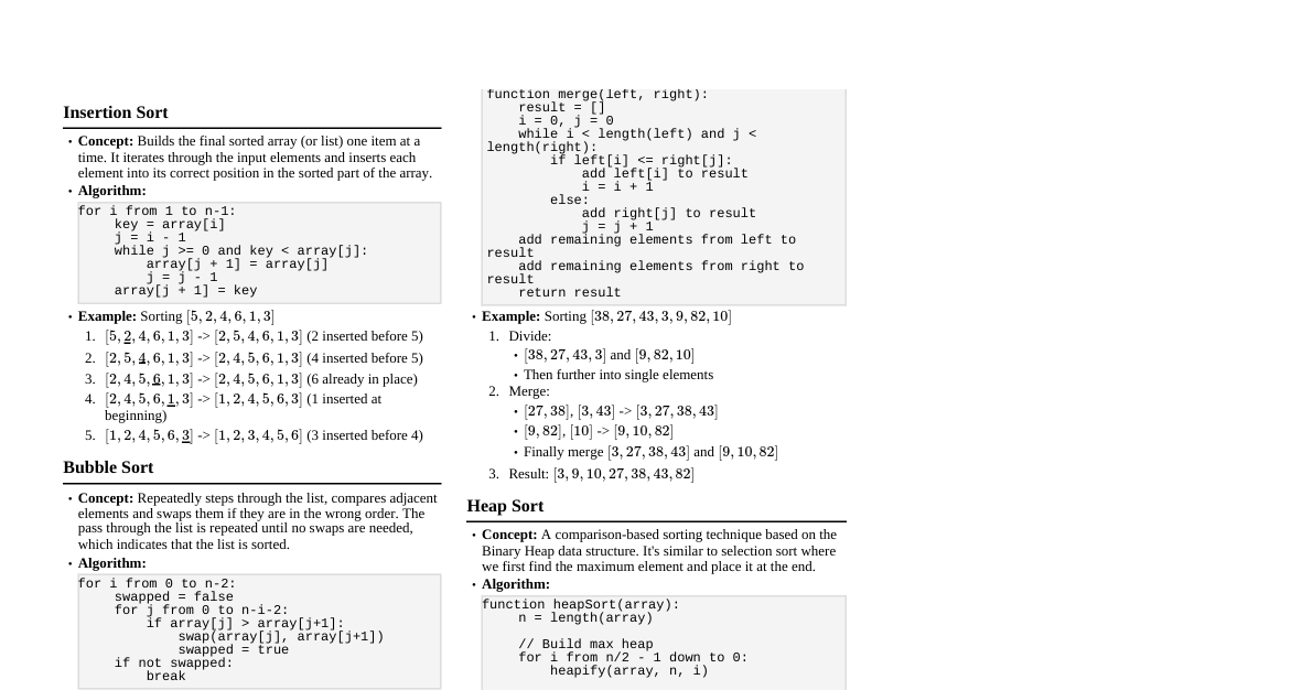
1. Asymptotic Notations Big O Notation ($O$): Upper bound. $O(g(n)) = \{f(n) : \exists c, n_0 > 0 \text{ s.t. } 0 \le f(n) \le c g(n) \text{ for all } n \ge n_0\}$. Omega Notation ($\Omega$): Lower bound. $\Omega(g(n)) = \{f(n) : \exists c, n_0 > 0 \text{ s.t. } 0 \le c g(n) \le f(n) \text{ for all } n \ge n_0\}$. Theta Notation ($\Theta$): Tight bound. $\Theta(g(n)) = \{f(n) : \exists c_1, c_2, n_0 > 0 \text{ s.t. } 0 \le c_1 g(n) \le f(n) \le c_2 g(n) \text{ for all } n \ge n_0\}$. Little o Notation ($o$): Strict upper bound. $f(n) = o(g(n))$ if $\lim_{n \to \infty} \frac{f(n)}{g(n)} = 0$. Little omega Notation ($\omega$): Strict lower bound. $f(n) = \omega(g(n))$ if $\lim_{n \to \infty} \frac{f(n)}{g(n)} = \infty$. 2. Recurrences 2.1. Substitution Method Guess the form of the solution. Use mathematical induction to find constants and prove the guess. Example: $T(n) = 2T(n/2) + n$. Guess $T(n) = O(n \log n)$. 2.2. Recursion-Tree Method Draw a tree representing the recursive calls and costs at each level. Sum costs at each level to get total cost. Useful for generating good guesses for the substitution method. 2.3. Master Method For recurrences of the form $T(n) = aT(n/b) + f(n)$, where $a \ge 1, b > 1$. If $f(n) = O(n^{\log_b a - \epsilon})$ for some $\epsilon > 0$, then $T(n) = \Theta(n^{\log_b a})$. If $f(n) = \Theta(n^{\log_b a})$, then $T(n) = \Theta(n^{\log_b a} \log n)$. If $f(n) = \Omega(n^{\log_b a + \epsilon})$ for some $\epsilon > 0$, and if $a f(n/b) \le c f(n)$ for some $c 3. Sorting Algorithms 3.1. Comparison Sorts (Lower Bound: $\Omega(n \log n)$) Insertion Sort: Time: $O(n^2)$ worst/average, $O(n)$ best. Space: $O(1)$. Stable. In-place. Good for nearly sorted or small arrays. Merge Sort: Time: $\Theta(n \log n)$ worst/average/best. Space: $O(n)$ (auxiliary array). Stable. Divide and Conquer. Recurrence: $T(n) = 2T(n/2) + \Theta(n)$. Heap Sort: Time: $\Theta(n \log n)$ worst/average/best. Space: $O(1)$. Not stable. In-place. Uses a max-heap. Build heap: $O(n)$. Extract max $n$ times: $O(n \log n)$. Quick Sort: Time: $O(n \log n)$ average/best, $O(n^2)$ worst. Space: $O(\log n)$ average, $O(n)$ worst (recursion stack). Not stable. In-place. Divide and Conquer. Pivot selection is critical. Randomized Quick Sort has $O(n \log n)$ expected time. 3.2. Non-Comparison Sorts Counting Sort: Time: $\Theta(n+k)$ where $k$ is range of input integers. Space: $\Theta(n+k)$. Stable. Requires integers in a small range. Radix Sort: Time: $\Theta(d(n+k))$ where $d$ is number of digits. Space: $\Theta(n+k)$. Stable. Sorts digits from least significant to most significant using a stable sort (e.g., Counting Sort). Bucket Sort: Time: $O(n)$ average (uniform distribution). Space: $O(n)$. Stable. Distributes elements into buckets, sorts each bucket, then concatenates. 4. Data Structures 4.1. Stacks and Queues Stack (LIFO): `PUSH`, `POP`, `PEEK`. All $O(1)$. Queue (FIFO): `ENQUEUE`, `DEQUEUE`, `FRONT`. All $O(1)$. 4.2. Linked Lists Singly, Doubly, Circular. Search: $O(n)$. Insert/Delete: $O(1)$ (given pointer to node). 4.3. Hash Tables Average Case: Insert, Delete, Search $O(1)$. Worst Case: $O(n)$. Collision Resolution: Chaining: Linked list at each slot. Open Addressing: Probing (linear, quadratic, double hashing). Load Factor ($\alpha$): $n/m$ (items/slots). Average search time $O(1+\alpha)$. 4.4. Binary Search Trees (BST) Search, Min, Max, Successor, Predecessor, Insert, Delete: $O(h)$ where $h$ is tree height. Worst case $h=O(n)$ (skewed tree). Best case $h=O(\log n)$ (balanced tree). 4.5. Red-Black Trees Self-balancing BST. Height is $O(\log n)$. Operations (Search, Min, Max, Insert, Delete): $O(\log n)$. Properties: Node is Red or Black. Root is Black. Leaves (NIL) are Black. Red node has Black children. All simple paths from node to descendant leaf contain same number of Black nodes. 4.6. B-Trees Balanced search trees for disk storage. Each node has many children. Height $O(\log_t n)$ where $t$ is minimum degree. Operations: $O(t \log_t n)$ or $O(\log_t n)$ disk I/Os. 4.7. Fibonacci Heaps Amortized time for many operations better than binary heaps. `MAKE-HEAP`: $O(1)$. `INSERT`: $O(1)$. `MINIMUM`: $O(1)$. `EXTRACT-MIN`: $O(\log n)$. `DECREASE-KEY`: $O(1)$. `DELETE`: $O(\log n)$. `UNION`: $O(1)$. 5. Graph Algorithms 5.1. Graph Representations Adjacency List: $O(V+E)$ space. Good for sparse graphs ($E \ll V^2$). Adjacency Matrix: $O(V^2)$ space. Good for dense graphs. Check edge existence in $O(1)$. 5.2. Graph Traversal Breadth-First Search (BFS): Finds shortest path in unweighted graphs. Time: $O(V+E)$. Uses a queue. Depth-First Search (DFS): Useful for topological sort, strongly connected components. Time: $O(V+E)$. Uses a stack (recursion). 5.3. Minimum Spanning Trees (MST) Prim's Algorithm: Time: $O(E \log V)$ with binary heap, $O(E + V \log V)$ with Fibonacci heap. Grows a single tree. Kruskal's Algorithm: Time: $O(E \log E)$ or $O(E \log V)$ (dominated by sorting edges). Uses Disjoint-Set data structure. Adds edges in increasing order of weight, avoiding cycles. 5.4. Single-Source Shortest Paths Bellman-Ford Algorithm: Handles negative edge weights. Detects negative cycles. Time: $O(VE)$. Dijkstra's Algorithm: Non-negative edge weights only. Time: $O(E \log V)$ with binary heap, $O(E + V \log V)$ with Fibonacci heap. 5.5. All-Pairs Shortest Paths Floyd-Warshall Algorithm: Time: $O(V^3)$. Handles negative edge weights. Dynamic Programming approach. Johnson's Algorithm: Time: $O(VE + V^2 \log V)$. Faster for sparse graphs. Uses Bellman-Ford to reweight edges, then V runs of Dijkstra. 5.6. Maximum Flow Ford-Fulkerson Method: Finds max flow in a flow network. Time: $O(E \cdot f_{max})$ where $f_{max}$ is max flow. Can be slow. Edmonds-Karp Algorithm: Specific implementation of Ford-Fulkerson using BFS to find augmenting paths. Time: $O(VE^2)$. 6. Dynamic Programming Optimal substructure: Optimal solution to problem contains optimal solutions to subproblems. Overlapping subproblems: Recursive algorithm revisits same subproblems repeatedly. Memoization (top-down) or Tabulation (bottom-up). Examples: Rod Cutting: $R_n = \max_{1 \le i \le n} (p_i + R_{n-i})$. Matrix Chain Multiplication: $m[i,j] = \min_{i \le k Longest Common Subsequence (LCS): If $x_i = y_j$, $c[i,j] = c[i-1,j-1] + 1$. Else, $c[i,j] = \max(c[i-1,j], c[i,j-1])$. 7. Greedy Algorithms Greedy choice property: A globally optimal solution can be reached by making locally optimal (greedy) choices. Optimal substructure. Examples: Activity Selection: Choose activity that finishes earliest. Huffman Coding: Build tree by repeatedly merging two lowest-frequency nodes. Fractional Knapsack: Take items with highest value-to-weight ratio. 8. Amortized Analysis Averages the time required to perform a sequence of operations over all the operations. Aggregate Analysis: Total time for $n$ operations is $T(n)$, average is $T(n)/n$. Accounting Method: Assign costs to operations, some operations "pay" for future expensive ones. Potential Method: Define a potential function $\Phi$. Amortized cost $\hat{c_i} = c_i + \Delta \Phi$. Examples: Dynamic arrays, Fibonacci Heaps. 9. NP-Completeness P: Class of problems solvable in polynomial time. NP: Class of problems whose solutions can be verified in polynomial time. NP-Hard: A problem $H$ is NP-hard if for every problem $L \in \text{NP}$, $L \le_P H$ (L is polynomial-time reducible to H). NP-Complete (NPC): A problem $C$ is NPC if $C \in \text{NP}$ and $C$ is NP-hard. To prove a problem $X$ is NP-complete: Prove $X \in \text{NP}$. Show $Y \le_P X$ for some known NPC problem $Y$. Examples of NPC problems: SAT, 3-SAT, Clique, Vertex Cover, Hamiltonian Cycle, Traveling Salesperson, Subset Sum, Knapsack.