Algorithms (CLRS)
Shared 3/31/2026•129 views
### Asymptotic Notation - **$O(g(n))$ (Big-O):** Upper bound. $f(n) \in O(g(n))$ if $\exists c, n_0 > 0$ such that $0 \le f(n) \le c g(n)$ for all $n \ge n_0$. - **$\Omega(g(n))$ (Big-Omega):** Lower bound. $f(n) \in \Omega(g(n))$ if $\exists c, n_0 > 0$ such that $0 \le c g(n) \le f(n)$ for all $n \ge n_0$. - **$\Theta(g(n))$ (Theta):** Tight bound. $f(n) \in \Theta(g(n))$ if $\exists c_1, c_2, n_0 > 0$ such that $0 \le c_1 g(n) \le f(n) \le c_2 g(n)$ for all $n \ge n_0$. - **$o(g(n))$ (Little-o):** Strict upper bound. $f(n) \in o(g(n))$ if $\lim_{n \to \infty} \frac{f(n)}{g(n)} = 0$. - **$\omega(g(n))$ (Little-omega):** Strict lower bound. $f(n) \in \omega(g(n))$ if $\lim_{n \to \infty} \frac{f(n)}{g(n)} = \infty$. ### Recursion: Master Theorem For recurrences of the form $T(n) = aT(n/b) + f(n)$, where $a \ge 1, b > 1$ are constants, $f(n)$ is asymptotically positive: 1. If $f(n) = O(n^{\log_b a - \epsilon})$ for some $\epsilon > 0$, then $T(n) = \Theta(n^{\log_b a})$. 2. If $f(n) = \Theta(n^{\log_b a})$, then $T(n) = \Theta(n^{\log_b a} \log n)$. 3. If $f(n) = \Omega(n^{\log_b a + \epsilon})$ for some $\epsilon > 0$, and if $a f(n/b) \le c f(n)$ for some $c ### Sorting Algorithms #### Insertion Sort - **Time Complexity:** $O(n^2)$ worst-case and average, $\Omega(n)$ best-case. - **Space Complexity:** $O(1)$ auxiliary. - **Stable:** Yes. - **In-place:** Yes. - **Use Case:** Small arrays or nearly sorted arrays. #### Merge Sort - **Time Complexity:** $\Theta(n \log n)$ in all cases. - **Space Complexity:** $O(n)$ auxiliary. - **Stable:** Yes. - **In-place:** No (requires extra space for merging). - **Recurrence:** $T(n) = 2T(n/2) + \Theta(n)$. #### Heap Sort - **Time Complexity:** $\Theta(n \log n)$ in all cases. - **Space Complexity:** $O(1)$ auxiliary. - **Stable:** No. - **In-place:** Yes. - **Process:** Build Max-Heap ($O(n)$), then repeatedly extract max ($O(\log n)$) $n$ times. #### Quick Sort - **Time Complexity:** $O(n \log n)$ average, $O(n^2)$ worst-case. - **Space Complexity:** $O(\log n)$ average (due to recursion stack), $O(n)$ worst-case. - **Stable:** No. - **In-place:** Yes (partitioning). - **Recurrence (worst):** $T(n) = T(0) + T(n-1) + \Theta(n) = T(n-1) + \Theta(n)$. - **Recurrence (best/average):** $T(n) = 2T(n/2) + \Theta(n)$. #### Counting Sort - **Time Complexity:** $\Theta(n+k)$ where $k$ is range of input numbers. - **Space Complexity:** $\Theta(n+k)$ auxiliary. - **Stable:** Yes. - **Use Case:** Non-comparison sort for integers in a small range. #### Radix Sort - **Time Complexity:** $\Theta(d(n+k))$ where $d$ is number of digits, $k$ is base. - **Space Complexity:** $\Theta(n+k)$ auxiliary. - **Stable:** Yes (if underlying sort is stable). - **Use Case:** Non-comparison sort for integers with many digits. #### Bucket Sort - **Time Complexity:** $O(n)$ average, $O(n^2)$ worst-case (if all items fall into one bucket). - **Space Complexity:** $\Theta(n+k)$ auxiliary. - **Use Case:** Uniformly distributed data. ### Graph Algorithms #### Breadth-First Search (BFS) - **Purpose:** Find shortest path in unweighted graph, traverse layers. - **Data Structure:** Queue. - **Time Complexity:** $O(V+E)$. - **Properties:** Finds shortest paths in terms of number of edges. #### Depth-First Search (DFS) - **Purpose:** Traverse graph, detect cycles, topological sort. - **Data Structure:** Stack (implicit via recursion). - **Time Complexity:** $O(V+E)$. - **Properties:** Explores as far as possible along each branch before backtracking. #### Dijkstra's Algorithm - **Purpose:** Find shortest paths from a single source to all other vertices in a graph with non-negative edge weights. - **Data Structure:** Min-priority queue. - **Time Complexity:** $O(E \log V)$ with binary heap, $O(E + V \log V)$ with Fibonacci heap. - **Greedy approach:** Always selects the vertex with the smallest shortest-path estimate. #### Bellman-Ford Algorithm - **Purpose:** Find shortest paths from a single source to all other vertices in a graph with possibly negative edge weights. Detects negative cycles. - **Time Complexity:** $O(VE)$. - **Properties:** Relaxes edges $|V|-1$ times. If a path can be further relaxed on the $|V|$-th iteration, a negative cycle exists. #### Floyd-Warshall Algorithm - **Purpose:** Find all-pairs shortest paths in a directed graph with positive or negative edge weights (no negative cycles). - **Dynamic Programming:** $d_{ij}^{(k)} = \min(d_{ij}^{(k-1)}, d_{ik}^{(k-1)} + d_{kj}^{(k-1)})$. - **Time Complexity:** $O(V^3)$. - **Space Complexity:** $O(V^2)$. #### Prim's Algorithm - **Purpose:** Find a Minimum Spanning Tree (MST) in an undirected, connected, weighted graph. - **Data Structure:** Min-priority queue. - **Time Complexity:** $O(E \log V)$ with binary heap, $O(E + V \log V)$ with Fibonacci heap. - **Greedy approach:** Grows MST from an arbitrary starting vertex. #### Kruskal's Algorithm - **Purpose:** Find a Minimum Spanning Tree (MST) in an undirected, connected, weighted graph. - **Data Structure:** Disjoint-set data structure. - **Time Complexity:** $O(E \log E)$ or $O(E \log V)$. - **Greedy approach:** Adds edges in increasing order of weight, avoiding cycles. #### Topological Sort - **Purpose:** Linear ordering of vertices in a Directed Acyclic Graph (DAG) such that for every directed edge $u \to v$, $u$ comes before $v$ in the ordering. - **Method:** DFS-based (order by finish times in decreasing order) or counting in-degrees. - **Time Complexity:** $O(V+E)$. ### Dynamic Programming - **Characteristics:** Optimal substructure and overlapping subproblems. - **Steps:** 1. Characterize optimal substructure. 2. Recursively define the value of an optimal solution. 3. Compute the value of an optimal solution (bottom-up or memoization). 4. Construct an optimal solution from computed information. #### Example: Rod Cutting - **Problem:** Given a rod of length $n$ and a table of prices $p_i$ for rods of length $i$, determine the maximum revenue obtainable by cutting up the rod and selling the pieces. - **Recurrence:** $r_n = \max_{1 \le i \le n} (p_i + r_{n-i})$, where $r_0 = 0$. #### Example: Longest Common Subsequence (LCS) - **Problem:** Find the longest subsequence common to two sequences. - **Recurrence:** Let $c[i,j]$ be the length of LCS of $X_i$ and $Y_j$. - If $x_i = y_j$: $c[i,j] = c[i-1, j-1] + 1$. - If $x_i \ne y_j$: $c[i,j] = \max(c[i-1, j], c[i, j-1])$. - **Time Complexity:** $O(mn)$ for sequences of length $m$ and $n$. #### Example: Matrix-Chain Multiplication - **Problem:** Given a sequence of matrices $A_1, A_2, ..., A_n$, find the most efficient way to multiply them. - **Recurrence:** $m[i,j] = \min_{i \le k ### Greedy Algorithms - **Characteristics:** Optimal substructure and greedy choice property. - **Steps:** 1. Cast the optimization problem as one where we make a choice. 2. Prove that there's always an optimal solution that makes the greedy choice. 3. Prove that all but one subproblem is empty (similar to dynamic programming, but simpler). #### Example: Activity Selection - **Problem:** Select maximum number of non-overlapping activities. - **Greedy Choice:** Always pick the activity that finishes earliest among the remaining compatible activities. - **Time Complexity:** $O(n \log n)$ if activities are not sorted by finish time, $O(n)$ if sorted. #### Example: Huffman Codes - **Problem:** Construct a prefix code for a given set of characters with given frequencies to minimize expected code length. - **Greedy Choice:** Combine the two lowest frequency nodes. - **Time Complexity:** $O(n \log n)$ where $n$ is number of characters. Uses a min-priority queue. ### Data Structures #### Hash Tables - **Direct-address table:** $O(1)$ search, insert, delete (if keys are small integers). - **Collision Resolution:** Chaining or Open Addressing (linear probing, quadratic probing, double hashing). - **Performance:** Average $O(1)$ search, insert, delete; worst-case $O(n)$. - **Load Factor:** $\alpha = n/m$. Average time is $O(1+\alpha)$. #### Binary Search Trees (BST) - **Properties:** Left child ### Maximum Flow - **Flow Network:** Directed graph $G=(V,E)$ with capacities $c(u,v) \ge 0$ and source $s$, sink $t$. - **Flow:** $f: V \times V \to \mathbb{R}$ satisfying: 1. **Capacity Constraint:** $f(u,v) \le c(u,v)$. 2. **Skew Symmetry:** $f(u,v) = -f(v,u)$. 3. **Flow Conservation:** $\sum_{v \in V} f(u,v) = 0$ for $u \ne s, t$. - **Value of Flow:** $|f| = \sum_{v \in V} f(s,v)$. - **Residual Network:** $G_f = (V, E_f)$ with residual capacities $c_f(u,v) = c(u,v) - f(u,v)$. - **Augmenting Path:** A path from $s$ to $t$ in the residual network. - **Ford-Fulkerson Method:** Repeatedly find augmenting paths and push flow. - **Edmonds-Karp Algorithm:** Uses BFS to find augmenting paths. Time: $O(VE^2)$. - **Max-Flow Min-Cut Theorem:** The value of a maximum $s-t$ flow is equal to the capacity of a minimum $s-t$ cut. ### String Matching #### Naive Algorithm - **Time Complexity:** $O((n-m+1)m)$, where $n$ is text length, $m$ is pattern length. #### Rabin-Karp Algorithm - **Approach:** Uses hashing to quickly find matches. - **Time Complexity:** Average $O(n+m)$, worst-case $O((n-m+1)m)$ (if many spurious hits). - **Hash function:** $h(P) = (p_k d^{k-1} + p_{k-1} d^{k-2} + ... + p_1 d^0) \mod q$. #### Knuth-Morris-Pratt (KMP) Algorithm - **Approach:** Uses a precomputed prefix function (LPS array) to avoid re-matching characters. - **Time Complexity:** $O(n+m)$. - **Prefix Function $\pi[q]$:** Length of the longest proper prefix of $P_q$ that is also a suffix of $P_q$. ### Computational Geometry #### Convex Hull - **Problem:** Smallest convex polygon enclosing a set of points. - **Algorithms:** - **Graham Scan:** $O(n \log n)$ (sorting by angle). - **Jarvis March (Gift Wrapping):** $O(nh)$ where $h$ is number of vertices on hull. - **Divide and Conquer:** $O(n \log n)$. #### Line Segment Intersection - **Problem:** Determine if any two segments in a set intersect. - **Bentley-Ottmann (Sweep-Line Algorithm):** $O(n \log n + k)$ where $k$ is number of intersections. ### NP-Completeness - **P (Polynomial Time):** Class of decision problems solvable in polynomial time. - **NP (Nondeterministic Polynomial Time):** Class of decision problems for which a "yes" instance can be verified in polynomial time. - **NP-Hard:** A problem $H$ is NP-hard if every problem $P \in NP$ can be polynomial-time reduced to $H$. - **NP-Complete:** A problem $C$ is NP-complete if $C \in NP$ and $C$ is NP-hard. - **Cook-Levin Theorem:** SAT (Boolean Satisfiability Problem) is NP-complete. - **Reductions:** $A \le_p B$ (A reduces to B) means if we can solve B in polynomial time, we can solve A in polynomial time. If $A \le_p B$ and $B \in P$, then $A \in P$. If $A \le_p B$ and $A$ is NP-hard, then $B$ is NP-hard.