Financial Management Essentials
Cheatsheet Content
1. Introduction to Financial Management Definition: Management of funds flow, focusing on financial decision-making. Objectives: Maximize shareholder wealth (primary), profit maximization (secondary). Key Concepts: Time Value of Money (TVM): A rupee today is worth more than a rupee tomorrow. Risk-Return Trade-off: Higher expected returns imply higher risk. Cash Flows: Focus on actual cash movements, not accounting profits. Core Decisions: Investment Decisions: Allocation of scarce resources to long-term assets (Capital Budgeting) and short-term assets (Working Capital Management). Financing Decisions: Determining optimal mix of debt and equity (Capital Structure). Dividend Decisions: How much profit to distribute to shareholders vs. retain for reinvestment. Relationship with Financial Accounting: Complementary; accounting provides data for financial management decisions. 2. Time Value of Money (TVM) Concept: Money received today is more valuable than the same amount received in the future due to earning potential and uncertainty. Techniques: Compounding: Calculating Future Value (FV). Single Sum: $FV = PV (1+r)^n$ Annuity (equal payments): $FV = PMT \times \frac{(1+r)^n - 1}{r}$ Discounting: Calculating Present Value (PV). Single Sum: $PV = \frac{FV}{(1+r)^n}$ Annuity: $PV = PMT \times \frac{1 - (1+r)^{-n}}{r}$ Perpetuity: $PV = \frac{PMT}{r}$ Growing Perpetuity: $PV = \frac{PMT_1}{r-g}$ (where $PMT_1$ is next period's payment) Effective Rate of Interest: Annualized rate when compounding occurs more than once a year. $ (1+r_e) = (1 + r/m)^m $ 3. Capital Budgeting: Introduction & Techniques 3.1. Introduction Definition: Decision-making process for long-term investments. Features: Long-term effects, substantial fund commitments, often irreversible, impact on firm's competitiveness. Key Principle: Focus on incremental after-tax cash flows, not accounting profits. Sunk Cost: Irrelevant, already incurred. Opportunity Cost: Relevant, value of best alternative foregone. Working Capital: Additional WC is an initial outflow, released WC is a terminal inflow. 3.2. Traditional Techniques (Non-Discounting) Payback Period (PB): Time to recover initial investment. Decision Rule: Accept if PB Pros: Simple, indicates liquidity. Cons: Ignores TVM, cash flows after payback, and total project life. Accounting Rate of Return (ARR): $\frac{\text{Average Annual Profit (after tax)}}{\text{Average Investment}} \times 100$ Decision Rule: Accept if ARR > target. Pros: Simple, uses accounting data. Cons: Ignores TVM, uses profits not cash flows, ignores project life. 3.3. Discounted Cash Flow (DCF) Techniques Net Present Value (NPV): $NPV = \sum_{i=0}^{n} \frac{CF_i}{(1+k)^i}$ Decision Rule: Accept if NPV > 0. Pros: Considers TVM, all cash flows, consistent with wealth maximization. Cons: Requires discount rate, absolute measure (size bias). Profitability Index (PI): $\frac{\text{PV of Cash Inflows}}{\text{PV of Cash Outflows}}$ Decision Rule: Accept if PI > 1. Pros: Relative measure (useful for capital rationing), considers TVM. Cons: May conflict with NPV for mutually exclusive projects. Internal Rate of Return (IRR): Discount rate $r$ such that $\sum_{i=0}^{n} \frac{CF_i}{(1+r)^i} = 0$. Decision Rule: Accept if IRR > cost of capital ($k$). Pros: Considers TVM, all cash flows, expressed as a percentage. Cons: Multiple IRRs possible, reinvestment rate assumption (IRR rate), complex calculation. Modified Internal Rate of Return (MIRR): Addresses IRR's reinvestment assumption by using the firm's cost of capital for reinvestment. 3.4. Risk Analysis in Capital Budgeting Risk-Adjusted Discount Rate (RADR): Adjusts the discount rate for project risk. Higher risk $\implies$ higher RADR. Certainty Equivalent (CE): Adjusts risky cash flows to equivalent certain cash flows, then discounts at risk-free rate. 4. Financing Decisions: Leverage Analysis Leverage: Responsiveness of one financial variable to changes in another. Operating Leverage (OL): Measures sensitivity of EBIT to sales changes. $OL = \frac{\% \Delta EBIT}{\% \Delta Sales} = \frac{Contribution}{EBIT}$ Arises from fixed operating costs. High OL implies high business risk. Financial Leverage (FL): Measures sensitivity of EPS to EBIT changes. $FL = \frac{\% \Delta EPS}{\% \Delta EBIT} = \frac{EBIT}{PBT}$ Arises from fixed financial charges (interest, preference dividends). High FL implies high financial risk. Combined Leverage (CL): Measures sensitivity of EPS to sales changes. $CL = OL \times FL = \frac{Contribution}{PBT}$ Represents total risk (business + financial). 5. Financing Decisions: EBIT-EPS Analysis & Capital Structure 5.1. EBIT-EPS Analysis Analyzes impact of different financing mixes on EPS at varying EBIT levels. Financial Break-even Level: EBIT level where EPS = 0. If only debt: $EBIT = \text{Interest Charge}$ If debt and preference shares: $EBIT = \text{Interest Charge} + \frac{\text{Pref. Div.}}{(1-t)}$ Indifference Point (EBIT): EBIT level where EPS from two different financing plans are equal. Limitations: Ignores risk factor (variability of EPS), focuses on short-term EPS rather than long-term wealth. 5.2. Theories of Capital Structure Assumptions: Only equity & debt, constant total assets, no retained earnings, constant operating profits, constant business risk, no taxes (initially). Net Income (NI) Approach: Capital structure matters. Assumes $k_d Increasing debt (cheaper source) decreases WACC and increases firm value ($V_F = V_E + V_D$). Net Operating Income (NOI) Approach: Capital structure does not matter. Assumes overall cost of capital ($k_0$) is constant. Increasing debt increases $k_e$ to exactly offset the benefit of cheaper debt, keeping $k_0$ and $V_F$ constant. ($V_F = EBIT / k_0$). Traditional Approach: A compromise view. Moderate debt increases firm value (WACC decreases) due to cheaper debt. Beyond a certain point, increased financial risk causes $k_e$ (and eventually $k_d$) to rise, increasing WACC and decreasing firm value. Suggests an optimal capital structure exists. Modigliani-Miller (MM) Hypothesis (without taxes): Supports NOI approach. Capital structure is irrelevant due to perfect capital markets and arbitrage. Arbitrage: Investors can create "homemade leverage" to replicate corporate leverage. MM Hypothesis (with taxes): Capital structure matters. Interest is tax-deductible, creating a tax shield. $V_L = V_U + \text{Debt} \times t$ (Levered firm value = Unlevered firm value + PV of tax shield). Debt financing increases firm value. 6. Cost of Capital Definition: Minimum required rate of return a firm must earn on its investments to maintain its value. Components: Risk-free rate ($I_f$), business risk premium, financial risk premium. After-Tax Cost: Most calculations are after-tax, especially for debt. Specific Costs: Debt ($k_d$): $k_d = \frac{I(1-t)}{B_0}$ (perpetual) or IRR-based (redeemable). Preference Shares ($k_p$): $k_p = \frac{PD}{P_0}$ (irredeemable) or IRR-based (redeemable). Equity ($k_e$): Dividend Growth Model: $k_e = \frac{D_1}{P_0} + g$ CAPM: $k_e = I_f + \beta (k_m - I_f)$ Retained Earnings ($k_r$): Opportunity cost, usually $k_r = k_e$. Weighted Average Cost of Capital (WACC): Overall cost of capital. $WACC = \sum (\text{Weight of Source} \times \text{Cost of Source})$ Weights can be book value or market value. Market value weights are theoretically preferred. Marginal Cost of Capital (MCC): Cost of raising an additional rupee of capital. 7. Dividend Decision & Valuation of the Firm Dividend Policy: Decision on what portion of profits to distribute vs. retain. Relevance Theories: Dividend policy affects firm value. Walter's Model: $P = \frac{D + (r/k_e)(E-D)}{k_e}$ If $r > k_e$ (growth firm), 0% payout maximizes value. If $r If $r = k_e$, dividend policy is irrelevant. Gordon's Model: $P = \frac{E(1-b)}{k_e - br}$ "Bird-in-the-hand" argument: Investors prefer certain current dividends over uncertain future capital gains. Similar conclusions to Walter's model. Irrelevance Theories: Dividend policy does not affect firm value. Residuals Theory: Dividends are a residual decision; paid only after all profitable investment opportunities are financed. Modigliani-Miller (MM) Hypothesis: $P_0 = \frac{1}{1+k_e} (D_1 + P_1)$ Assumes perfect capital markets, no taxes, no transaction costs. Arbitrage process ensures firm value is independent of dividend policy. Dividend Payout Ratio: Percentage of earnings distributed as dividends. Stability of Dividends: Consistent dividend payments are generally favored by investors. Bonus Shares (Stock Dividends): Issue of additional shares from capitalized reserves; no cash outflow. Increases number of shares, reduces EPS and market price per share, but total wealth should be constant. Signals positive future prospects. Informational Content of Dividends: Unexpected changes in dividends can signal management's view of future earnings. 8. Working Capital: Planning & Management Definition: Management of current assets (cash, inventory, receivables) and current liabilities. Gross Working Capital: Total investment in current assets. Net Working Capital: Current Assets - Current Liabilities. Indicates liquidity. Operating Cycle: Time from raw material procurement to cash realization from sales. $Operating\ Cycle = \text{Raw Material Conversion Period} + \text{Work-in-Progress Conversion Period} + \text{Finished Goods Conversion Period} + \text{Receivables Conversion Period} - \text{Deferral Period}$ Shorter cycle $\implies$ less working capital needed. Factors Affecting Working Capital: Nature of business, business cycle, seasonal operations, market competitiveness, credit policy, supply conditions. Risk-Return Trade-off: Higher working capital $\implies$ higher liquidity, lower profitability (and vice-versa). Types of Working Capital: Permanent: Minimum level required at all times. Temporary: Seasonal/fluctuating needs above permanent level. Financing Approaches: Hedging (Matching): Match asset maturity with financing maturity (long-term for permanent, short-term for temporary). Conservative: Finance all or most working capital with long-term sources (low risk, low return). Aggressive: Finance part of permanent working capital with short-term sources (high risk, high return). 9. Cash Management Motives for Holding Cash: Transactionary, Precautionary, Speculative, Compensation. Objectives: Meet cash outflows, optimize cash balance (minimize idle cash). Cash Budget: Forecast of cash inflows and outflows over a period. Helps identify surpluses/deficits. Managing Float: Difference between bank balance and book balance. Payment Float: Checks issued but not yet cleared. Receipt Float: Checks received and deposited but not yet cleared. Techniques: Concentration banking, lock-box systems to reduce receipt float. Optimal Cash Balance Models: Baumol's Model: $EOQ_{\text{cash}} = \sqrt{\frac{2FT}{r}}$ (balances transaction cost and holding cost). Miller-Orr Model: Sets upper and lower control limits for cash balance, with a "return point" to which cash is restored. Marketable Securities: Short-term liquid investments for surplus cash. Key considerations: Maturity, liquidity, default risk, yield. 10. Receivables Management Definition: Managing credit extended to customers (accounts receivable). Costs: Financing costs, administrative costs, delinquency costs, bad debts. Benefits: Increased sales and profits. Credit Policy: Set of parameters for extending credit. Credit Standards: Criteria for granting credit (character, capacity, capital, collateral, conditions). Credit Terms: Credit period, cash discounts offered (e.g., 2/10 net 30). Annualized Cost of Cash Discount: $\frac{\text{Discount \%}}{100 - \text{Discount \%}} \times \frac{365}{\text{Credit Period - Discount Period}}$ Credit Evaluation: Assessing customer creditworthiness through various information sources. Credit Control: Procedures for timely collection and monitoring. Average Collection Period: $\frac{\text{Average Receivables}}{\text{Credit Sales per day}}$ Ageing Schedule: Classifying receivables by age to identify overdue accounts. Lines of Credit: Maximum credit limit for each customer. Evaluation of Credit Policies: Compare incremental benefits (increased contribution) against incremental costs (financing, bad debts, collection). 11. Inventory Management Types of Inventories: Raw materials, work-in-progress, finished goods. Reasons for Inventories: Transactionary, precautionary, speculative motives; uninterrupted production/sales. Costs of Inventory: Carrying Costs: Storage, insurance, obsolescence, opportunity cost of capital. Ordering Costs: Placing and receiving an order. Stock-out Costs: Lost sales, production delays, loss of goodwill. Objective: Minimize total inventory costs while ensuring smooth operations. Techniques: ABC Analysis: Classifies inventory items by value (A-high value, B-medium, C-low) to prioritize management effort. Economic Order Quantity (EOQ) Model: $EOQ = \sqrt{\frac{2AO}{C}}$ A = Annual demand, O = Ordering cost per order, C = Carrying cost per unit per annum. Minimizes total ordering and carrying costs. Re-order Level: Inventory level at which a new order is placed. $R = M + tU$ (M=min level, t=lead time, U=usage rate). Safety Stock: Buffer inventory to guard against unexpected demand or delays. Quantity Discounts: Evaluate if savings from discount outweigh increased carrying costs. 12. Valuation of Securities Concept: Determining the worth of an asset (financial assets here). Economic Value (Capitalized Value): Present value of all future cash flows, discounted at a rate commensurate with risk. $V_0 = \sum_{i=1}^{n} \frac{CF_i}{(1+k)^i}$ Required Rate of Return ($k$): $k = I_f + r_p$ (Risk-free rate + Risk premium). Bond Valuation: $B_0 = \sum_{i=1}^{n} \frac{I}{(1+k_d)^i} + \frac{RV}{(1+k_d)^n}$ Yield to Maturity (YTM): The discount rate $k_d$ that equates the bond's present value to its current market price. Convertible Debentures: Value depends on interest payments, share price at conversion, and redemption amount. Deep Discount Bonds (DDB): Zero-coupon bonds, valued as PV of face value at maturity. Preference Share Valuation: Redeemable: Similar to bond valuation, using fixed dividends and redemption value. Irredeemable: $P_0 = \frac{D}{k_p}$ (perpetuity). Equity Share Valuation: More complex due to uncertain dividends and no maturity. Accounting Information: Book Value, Liquidation Value (less common for investment decisions). Dividends-Based Models: Zero Growth (Constant Dividends): $P_0 = \frac{D}{k_e}$ Constant Growth (Gordon Growth Model): $P_0 = \frac{D_1}{k_e - g}$ Variable Growth: Sum of PV of dividends during variable growth phases + PV of terminal value (constant growth phase). Earnings-Based Models: P/E Ratio Approach: $\text{Value} = EPS \times P/E\ \text{Ratio}$ Gordon's and Walter's models (also consider earnings and reinvestment).