Introduction to Algorithms (CL
Cheatsheet Content
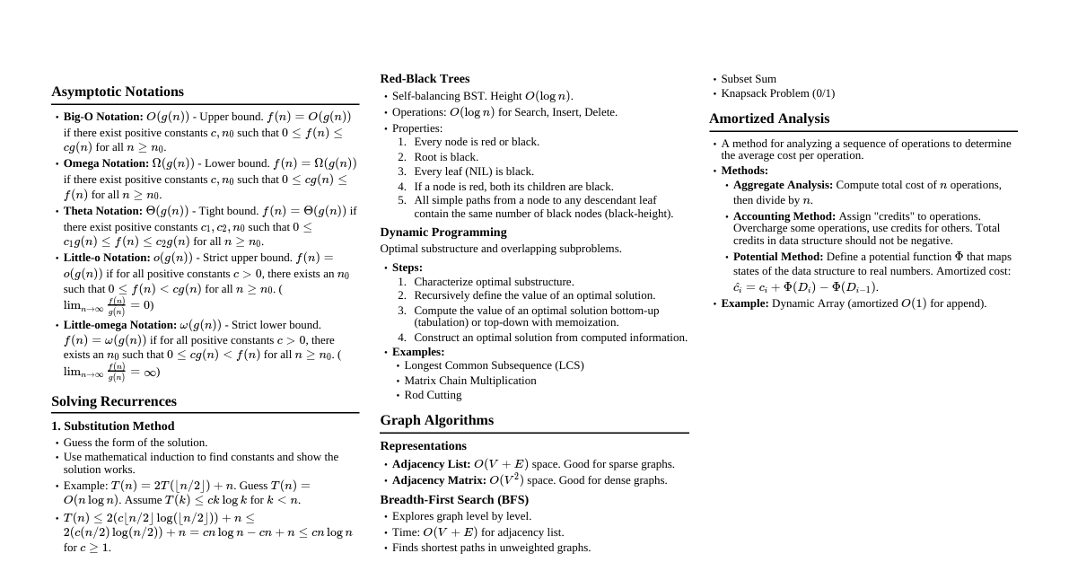
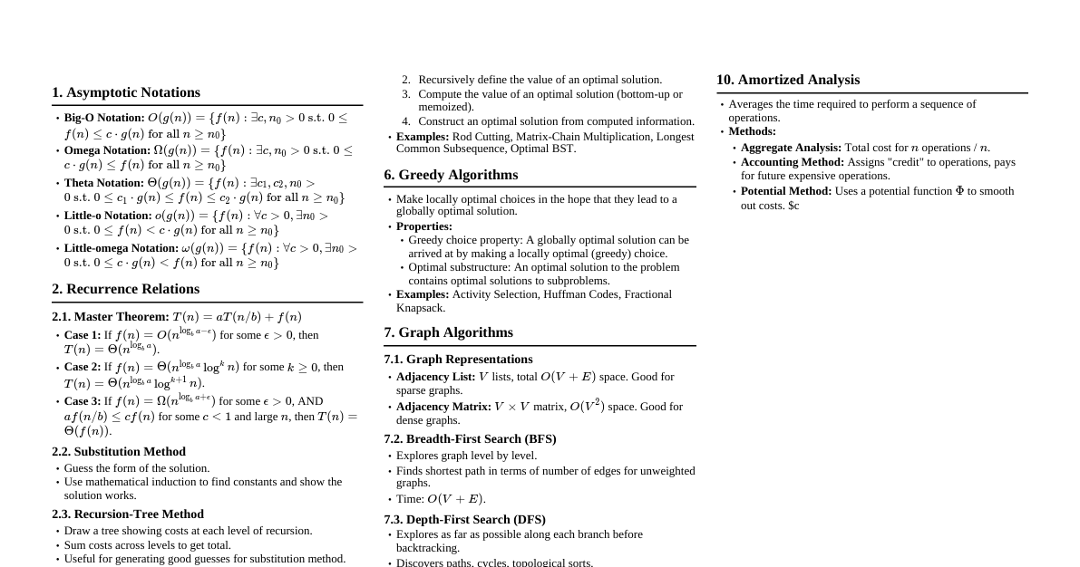
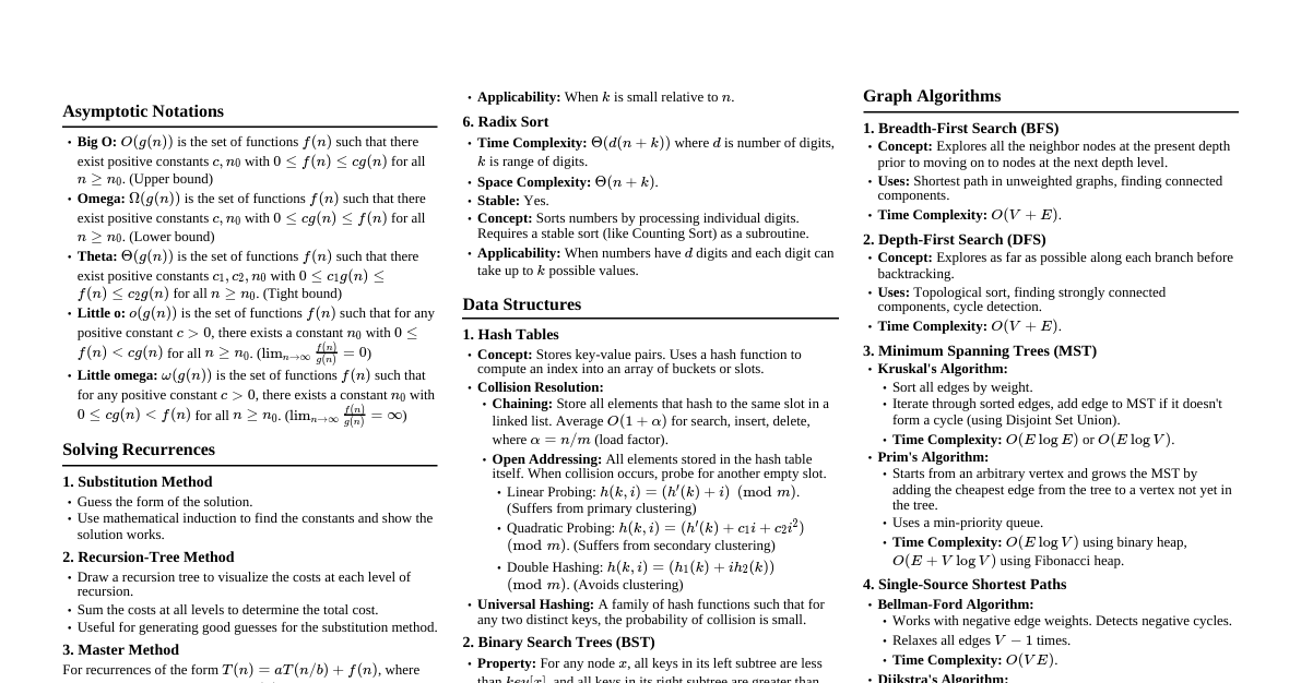
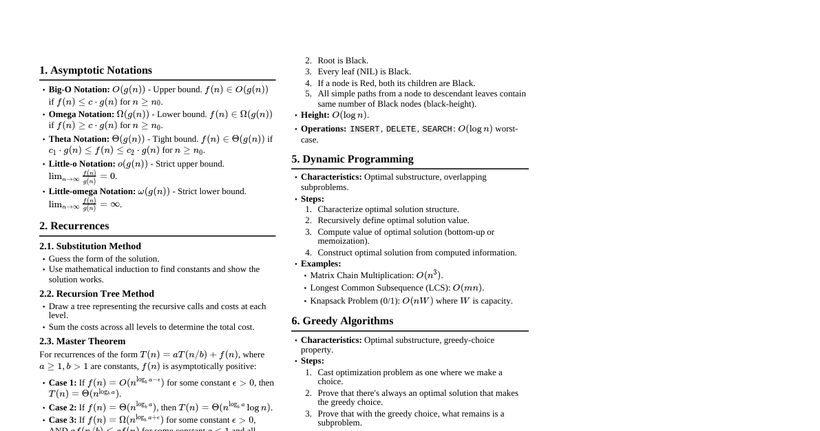
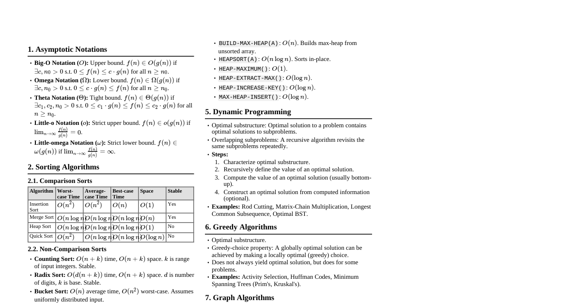
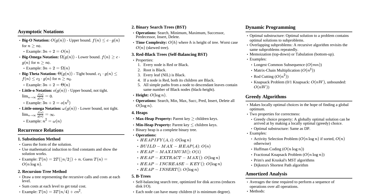
### Asymptotic Notation - **Big O ($O$)**: Upper bound. $f(n) = O(g(n))$ if $f(n) \le c \cdot g(n)$ for all $n \ge n_0$. - **Omega ($\Omega$)**: Lower bound. $f(n) = \Omega(g(n))$ if $f(n) \ge c \cdot g(n)$ for all $n \ge n_0$. - **Theta ($\Theta$)**: Tight bound. $f(n) = \Theta(g(n))$ if $c_1 \cdot g(n) \le f(n) \le c_2 \cdot g(n)$ for all $n \ge n_0$. - **Little o ($o$)**: Strict upper bound. $f(n) = o(g(n))$ if $\lim_{n \to \infty} \frac{f(n)}{g(n)} = 0$. - **Little omega ($\omega$)**: Strict lower bound. $f(n) = \omega(g(n))$ if $\lim_{n \to \infty} \frac{f(n)}{g(n)} = \infty$. #### Properties - Transitivity: If $f(n) = O(g(n))$ and $g(n) = O(h(n))$, then $f(n) = O(h(n))$. - Reflexivity: $f(n) = O(f(n))$. - Symmetry: $f(n) = \Theta(g(n))$ iff $g(n) = \Theta(f(n))$. ### Divide and Conquer - **General Method:** 1. **Divide:** Break the problem into subproblems. 2. **Conquer:** Solve the subproblems recursively. 3. **Combine:** Combine subproblem solutions into the main problem solution. - **Master Theorem:** For recurrences of the form $T(n) = aT(n/b) + f(n)$: 1. If $f(n) = O(n^{\log_b a - \epsilon})$ for some $\epsilon > 0$, then $T(n) = \Theta(n^{\log_b a})$. 2. If $f(n) = \Theta(n^{\log_b a})$, then $T(n) = \Theta(n^{\log_b a} \log n)$. 3. If $f(n) = \Omega(n^{\log_b a + \epsilon})$ for some $\epsilon > 0$, and $af(n/b) \le cf(n)$ for some $c ### Sorting Algorithms | Algorithm | Avg. Case Time | Worst Case Time | Space | Stable | Notes | |----------------|----------------|-----------------|-------|--------|-----------------------------------------| | Insertion Sort | $\Theta(n^2)$ | $\Theta(n^2)$ | $O(1)$| Yes | Good for small arrays/nearly sorted | | Merge Sort | $\Theta(n \log n)$ | $\Theta(n \log n)$| $O(n)$| Yes | Guaranteed $O(n \log n)$ | | Heap Sort | $\Theta(n \log n)$ | $\Theta(n \log n)$| $O(1)$| No | In-place, uses Max-Heap | | Quick Sort | $\Theta(n \log n)$ | $\Theta(n^2)$ | $O(\log n)$| No | Fastest in practice (avg case) | | Counting Sort | $\Theta(n+k)$ | $\Theta(n+k)$ | $O(n+k)$| Yes | For integers in range $[0, k]$ | | Radix Sort | $\Theta(d(n+k))$| $\Theta(d(n+k))$| $O(n+k)$| Yes | For integers with $d$ digits, base $k$ | #### Comparison Sort Lower Bound - Any comparison sort requires $\Omega(n \log n)$ comparisons in the worst case. ### Dynamic Programming - **Method:** 1. Characterize optimal substructure. 2. Recursively define the value of an optimal solution. 3. Compute the value of an optimal solution (typically bottom-up). 4. Construct an optimal solution from computed information. - **Overlapping Subproblems:** Solutions to subproblems are reused. - **Optimal Substructure:** Optimal solution to a problem contains optimal solutions to subproblems. #### Examples - **Longest Common Subsequence (LCS):** - $c[i,j]$ = length of LCS of $X[1..i]$ and $Y[1..j]$. - If $x_i = y_j$, $c[i,j] = c[i-1,j-1] + 1$. - If $x_i \ne y_j$, $c[i,j] = \max(c[i-1,j], c[i,j-1])$. - **Matrix Chain Multiplication:** - $m[i,j]$ = min scalar multiplications to compute $A_i \dots A_j$. - $m[i,j] = \min_{i \le k ### Greedy Algorithms - **Method:** Make locally optimal choices in the hope of finding a globally optimal solution. - **Properties:** - **Greedy-choice property:** A globally optimal solution can be reached by making a locally optimal (greedy) choice. - **Optimal substructure:** An optimal solution to the problem contains optimal solutions to its subproblems. #### Examples - **Activity Selection Problem:** Select maximum number of non-overlapping activities. - Sort activities by finish time. Pick the first activity, then pick the next non-overlapping activity. - **Huffman Coding:** Construct optimal prefix codes. - Repeatedly merge two trees with smallest frequencies. ### Graph Algorithms #### Representations - **Adjacency List:** $O(V+E)$ space. Good for sparse graphs. - **Adjacency Matrix:** $O(V^2)$ space. Good for dense graphs. #### Breadth-First Search (BFS) - Finds shortest paths in unweighted graphs. - Time: $O(V+E)$. #### Depth-First Search (DFS) - Used for topological sort, strongly connected components. - Time: $O(V+E)$. #### Minimum Spanning Trees (MST) - **Prim's Algorithm:** Starts from a vertex, grows the MST by adding the cheapest edge to a vertex in the MST. $O(E \log V)$ with Fibonacci heap, $O(E \log V)$ with binary heap. - **Kruskal's Algorithm:** Sorts all edges by weight, adds edges if they don't form a cycle. $O(E \log E)$ or $O(E \log V)$ using a disjoint-set data structure. #### Shortest Paths - **Dijkstra's Algorithm (Single-Source, Non-Negative Weights):** - Uses a priority queue. $O(E \log V)$ with binary heap. - **Bellman-Ford Algorithm (Single-Source, General Weights):** - Detects negative cycles. $O(VE)$. - **Floyd-Warshall Algorithm (All-Pairs, General Weights):** - $O(V^3)$. ### Data Structures #### Hash Tables - Average $O(1)$ search, insert, delete. Worst case $O(n)$. - **Collision Resolution:** Chaining, Open Addressing (Linear Probing, Quadratic Probing, Double Hashing). #### Binary Search Trees (BST) - Average $O(h)$ for search, insert, delete, where $h$ is height. Worst case $O(n)$. - Inorder traversal yields sorted elements. #### Red-Black Trees (Self-Balancing BST) - Guarantees $O(\log n)$ for search, insert, delete operations. - Properties: 1. Node is Red or Black. 2. Root is Black. 3. Leaves (NIL) are Black. 4. If node is Red, both children are Black. 5. All paths from node to descendant NIL leaves have same number of Black nodes. #### Heaps (Binary Heap) - Max-Heap or Min-Heap. - Operations: `INSERT`, `MAXIMUM`, `EXTRACT-MAX`, `INCREASE-KEY`. All $O(\log n)$. - Build Heap: $O(n)$. #### Disjoint-Set Data Structure - Operations: `MAKE-SET`, `FIND-SET`, `UNION`. - Path compression and union by rank/size give nearly constant time complexity (amortized $O(\alpha(n))$). ### String Matching - **Naive Algorithm:** $O((n-m+1)m)$. - **Rabin-Karp Algorithm:** Uses hashing. Average $O(n+m)$, worst case $O((n-m+1)m)$. - **Knuth-Morris-Pratt (KMP) Algorithm:** Uses a prefix function to avoid redundant comparisons. $O(n+m)$. ### NP-Completeness - **P (Polynomial time):** Problems solvable in polynomial time. - **NP (Nondeterministic Polynomial time):** Problems whose solutions can be verified in polynomial time. - **NP-Hard:** A problem $H$ is NP-hard if every problem $L \in NP$ can be polynomial-time reduced to $H$. - **NP-Complete:** A problem $C$ is NP-complete if $C \in NP$ and $C$ is NP-hard. #### Common NP-Complete Problems - Satisfiability (SAT) - Traveling Salesperson Problem (TSP) - Vertex Cover - Hamiltonian Cycle - Clique