Mathematics Notes
Cheatsheet Content
1. Matrices 1.1 Definition of a Matrix Definition 1.1.1 (Matrix): A rectangular array of numbers. Rows: Horizontal arrays. Columns: Vertical arrays. Order: An $m \times n$ matrix has $m$ rows and $n$ columns. Entry: $a_{ij}$ is the entry at the intersection of the $i^{th}$ row and $j^{th}$ column. Column Vector: A matrix with only one column. Row Vector: A matrix with only one row. Definition 1.1.3 (Equality of two Matrices): Two matrices $A = [a_{ij}]$ and $B = [b_{ij}]$ of the same order $m \times n$ are equal if $a_{ij} = b_{ij}$ for all $i, j$. 1.1.1 Special Matrices Definition 1.1.5: Zero-matrix ($0$): All entries are zero. Square matrix: Number of rows equals number of columns ($m \times m$ or order $m$). Diagonal entries: For a square matrix $A = [a_{ij}]$ of order $n$, entries $a_{11}, a_{22}, ..., a_{nn}$ form the principal diagonal. Diagonal matrix: A square matrix $A = [a_{ij}]$ where $a_{ij} = 0$ for $i \neq j$. Denoted $D = \text{diag}(d_1, ..., d_n)$. Scalar matrix: A diagonal matrix $D$ where $d_i = d$ for all $i$. Identity matrix ($I_n$): A square matrix $A = [a_{ij}]$ where $a_{ij} = 1$ if $i=j$ and $a_{ij} = 0$ if $i \neq j$. Upper triangular matrix: A square matrix $A = [a_{ij}]$ where $a_{ij} = 0$ for $i > j$. Lower triangular matrix: A square matrix $A = [a_{ij}]$ where $a_{ij} = 0$ for $i Triangular matrix: An upper or lower triangular matrix. 1.2 Operations on Matrices Definition 1.2.1 (Transpose of a Matrix): For an $m \times n$ matrix $A = [a_{ij}]$, its transpose $A^t$ is an $n \times m$ matrix $B = [b_{ij}]$ with $b_{ij} = a_{ji}$. Theorem 1.2.2: For any matrix $A$, $(A^t)^t = A$. Definition 1.2.3 (Addition of Matrices): For $A = [a_{ij}]$ and $B = [b_{ij}]$ of the same order $m \times n$, $A+B = [a_{ij}+b_{ij}]$. Definition 1.2.4 (Multiplying a Scalar to a Matrix): For an $m \times n$ matrix $A = [a_{ij}]$ and scalar $k \in \mathbb{R}$, $kA = [ka_{ij}]$. Theorem 1.2.5: For $A, B, C$ of order $m \times n$, and $k, l \in \mathbb{R}$: $A+B = B+A$ (commutativity). $(A+B)+C = A+(B+C)$ (associativity). $k(lA) = (kl)A$. $(k+l)A = kA+lA$. Definition 1.2.7 (Additive Inverse): For an $m \times n$ matrix $A$, $-A = (-1)A$ is its additive inverse. The zero matrix $O_{m \times n}$ is the additive identity. 1.2.1 Multiplication of Matrices Definition 1.2.8 (Matrix Multiplication / Product): For an $m \times n$ matrix $A = [a_{ij}]$ and an $n \times r$ matrix $B = [b_{ij}]$, the product $AB$ is an $m \times r$ matrix $C = [c_{ij}]$ with $c_{ij} = \sum_{k=1}^n a_{ik}b_{kj}$. Defined if number of columns of A = number of rows of B. Definition 1.2.9 (Commute): Two square matrices $A$ and $B$ commute if $AB = BA$. Remark 1.2.10: $A I_n = I_n A$. Matrix product is generally not commutative. Theorem 1.2.11: For matrices $A, B, C$ (where multiplications are defined) and $k \in \mathbb{R}$: $(AB)C = A(BC)$ (associativity). $(kA)B = k(AB) = A(kB)$. $A(B+C) = AB+AC$ (distributivity). $A I_n = I_n A = A$. For square matrix $A$ of order $n$ and $D = \text{diag}(d_1, ..., d_n)$: First row of $DA$ is $d_1$ times the first row of $A$. $i^{th}$ row of $DA$ is $d_i$ times the $i^{th}$ row of $A$. Exercise 1.2.12: $(A+B)^t = A^t+B^t$. If $AB$ is defined, $(AB)^t = B^t A^t$. 1.3 Some More Special Matrices Definition 1.3.1: Symmetric: $A^t = A$. Skew-symmetric: $A^t = -A$. Orthogonal: $AA^t = A^t A = I$. Definition 1.1.5 (continued): Nilpotent matrix: A square matrix $A$ where $A^k = 0$ for some positive integer $k$. The least such $k$ is the order of nilpotency. Idempotent matrix: A square matrix $A$ where $A^2 = A$. 1.3.1 Submatrix of a Matrix Definition 1.3.4 (Submatrix): A matrix obtained by deleting some rows and/or columns. Theorem 1.3.6 (Block Matrices): If $A = [P \quad Q]$ and $B = \begin{pmatrix} H \\ K \end{pmatrix}$, then $AB = PH + QK$. 1.4 Matrices over Complex Numbers Definition 1.4.1 (Conjugate Transpose of a Matrix): For an $m \times n$ matrix $A = [a_{ij}]$ over $\mathbb{C}$: Conjugate of A ($\bar{A}$): Matrix $B = [b_{ij}]$ with $b_{ij} = \bar{a}_{ij}$. Conjugate Transpose of A ($A^*$): Matrix $B = [b_{ij}]$ with $b_{ij} = \bar{a}_{ji}$. Hermitian: $A^* = A$. Skew-Hermitian: $A^* = -A$. Unitary: $A^*A = AA^* = I$. Normal: $AA^* = A^*A$. Remark 1.4.2: If $A = [a_{ij}]$ with $a_{ij} \in \mathbb{R}$, then $A^* = A^t$. 2. Linear System of Equations 2.1 Introduction Linear systems can have: Unique solution. Infinite number of solutions. No solution. 2.2 Definition and a Solution Method Definition 2.2.1 (Linear System): A set of $m$ equations in $n$ unknowns $x_1, ..., x_n$. $$a_{11}x_1 + \dots + a_{1n}x_n = b_1$$ $$\vdots$$ $$a_{m1}x_1 + \dots + a_{mn}x_n = b_m$$ Homogeneous: If $b_1 = \dots = b_m = 0$. Non-homogeneous: Otherwise. Matrix Form: $Ax = b$, where $A$ is the coefficient matrix, $x$ is the vector of unknowns, and $b$ is the constant vector. Augmented Matrix: $[A \mid b]$. Remark 2.2.2: $i^{th}$ row of $[A \mid b]$ represents $i^{th}$ equation. $j^{th}$ column of $A$ corresponds to coefficients of $j^{th}$ variable $x_j$. Associated Homogeneous System: $Ax = 0$. Definition 2.2.3 (Solution): A column vector $y = [y_1, ..., y_n]^t$ such that $Ay = b$. Trivial Solution: $x=0$ for $Ax=0$. Non-trivial Solution: Non-zero $x$ for $Ax=0$. 2.3 Row Operations and Equivalent Systems Definition 2.3.1 (Elementary Operations): Interchange two equations. Multiply an equation by a non-zero constant. Replace an equation by itself plus a constant multiple of another equation. Inverse Operations: Each elementary operation has an inverse operation. Definition 2.3.2 (Equivalent Linear Systems): Two linear systems are equivalent if one can be obtained from the other by a finite number of elementary operations. Lemma 2.3.3: If $Cx=d$ is obtained from $Ax=b$ by an elementary operation, then $Ax=b$ and $Cx=d$ have the same set of solutions. Theorem 2.3.4: Two equivalent systems have the same set of solutions. 2.3.1 Gauss Elimination Method Definition 2.3.5 (Elementary Row Operations): Interchange $i^{th}$ and $j^{th}$ rows ($R_{ij}$). Multiply $k^{th}$ row by $c \neq 0$ ($R_k(c)$). Replace $k^{th}$ row by $k^{th}$ row plus $c$ times $j^{th}$ row ($R_{kj}(c)$). Exercise 2.3.6: Find inverse row operations. Definition 2.3.7 (Row Equivalent Matrices): Two matrices are row-equivalent if one can be obtained from the other by a finite number of elementary row operations. Definition 2.3.9 (Forward/Gauss Elimination Method): Method of solving $Ax=b$ by bringing augmented matrix $[A \mid b]$ to upper triangular form. 2.4 Row Reduced Echelon Form of a Matrix Definition 2.4.1 (Row Reduced Form): A matrix $C$ is in row reduced form if: First non-zero entry in each row is 1. Column containing this 1 has all other entries zero. Definition 2.4.3 (Leading Term, Leading Column): For a row-reduced matrix, the first non-zero entry of any row is a leading term. Columns containing leading terms are leading columns. Definition 2.4.4 (Basic, Free Variables): In $Ax=b$, variables corresponding to leading columns in first $n$ columns of row-reduced $[C \mid d]$ are basic variables. Others are free variables. Remark 2.4.5: If there are $r$ non-zero rows in row-reduced form, there are $r$ leading terms, $r$ basic variables, and $n-r$ free variables. 2.4.1 Gauss-Jordan Elimination Definition 2.4.6 (Row Reduced Echelon Form): A matrix $C$ is in row reduced echelon form if: It is already in row reduced form. Rows consisting of all zeros come below all non-zero rows. Leading terms appear from left to right in successive rows. Method to get row-reduced echelon form: Steps 1-5 (detailed in original document). Remark 2.4.10: Row reduction involves only row operations and proceeds from left to right. Theorem 2.4.11: The row reduced echelon form of a matrix is unique. 2.4.2 Elementary Matrices Definition 2.4.13 (Elementary Matrix): A square matrix $E$ of order $n$ obtained by applying exactly one elementary row operation to $I_n$. Remark 2.4.14: Three types of elementary matrices correspond to the three elementary row operations ($R_{ij}$, $R_k(c)$, $R_{kj}(c)$). Left multiplication by an elementary matrix performs a row operation. Definition 2.4.16 (Elementary Column Operations): Column transformations obtained by right multiplication of elementary matrices. 2.5 Rank of a Matrix Definition 2.5.1 (Consistent, Inconsistent): A linear system is consistent if it admits a solution, inconsistent otherwise. Definition 2.5.2 (Row rank of a Matrix): The number of non-zero rows in the row reduced form of a matrix. Denoted $\text{row-rank}(A)$. Remark 2.5.4: $\text{row-rank}(A) \le \text{row-rank}([A \mid b])$. Remark 2.5.5 (Column rank): Number of non-zero columns in the matrix $B$ obtained by applying elementary column operations, where $B$ has properties detailed in document. $\text{row-rank}(A) = \text{column-rank}(A)$. Definition 2.5.6 (Rank of a Matrix): The number of non-zero rows in the row reduced form of a matrix $A$. Denoted $\text{rank}(A)$. Theorem 2.5.7: If $A$ is a matrix of rank $r$, there exist elementary matrices $E_1, \dots, E_s$ and $F_1, \dots, F_e$ such that $E_1 \dots E_s A F_1 \dots F_e = \begin{pmatrix} I_r & 0 \\ 0 & 0 \end{pmatrix}$. 2.6 Existence of Solution of $Ax=b$ Theorem 2.6.1 (Existence and Non-existence): For linear system $Ax=b$ with $A$ an $m \times n$ matrix, $x,b$ vectors, $\text{rank}(A)=r$, $\text{rank}([A \mid b])=r_a$: If $r_a = r If $r_a = r = n$, unique solution $x_0$. If $r Remark 2.6.2: $Ax=b$ is consistent if and only if $\text{rank}(A) = \text{rank}([A \mid b])$. Corollary 2.6.3: Homogeneous system $Ax=0$ has a non-trivial solution if and only if $\text{rank}(A) Proposition 2.6.4: For $Ax=b$: "unique solution for every $b$" and "$Ax=0$ has non-trivial solution" cannot hold together. Remark 2.6.5: If $x_1, x_2$ are solutions of $Ax=0$, then $k_1x_1+k_2x_2$ is also a solution. If $u, v$ are solutions of $Ax=b$, then $u-v$ is a solution of $Ax=0$. For $b \neq 0$, solutions of $Ax=b$ are $\{x_0+x_h\}$, where $x_0$ is a particular solution and $x_h$ is a solution of $Ax=0$. 2.7 Invertible Matrices 2.7.1 Inverse of a Matrix Definition 2.7.1 (Inverse of a Matrix): For square matrix $A$ of order $n$: Left Inverse ($B$): $BA = I_n$. Right Inverse ($C$): $AC = I_n$. Invertible (Inverse): Exists $B$ such that $AB=BA=I_n$. Lemma 2.7.2: If $AB=I_n$ and $CA=I_n$, then $B=C$. Remark 2.7.3: Inverse of $A$ is unique, denoted $A^{-1}$. Theorem 2.7.4: For invertible matrices $A, B$: $(A^{-1})^{-1} = A$. $(AB)^{-1} = B^{-1}A^{-1}$. $(A^t)^{-1} = (A^{-1})^t$. 2.7.2 Equivalent conditions for Invertibility Definition 2.7.6 (Full Rank): A square matrix $A$ of order $n$ has full rank if $\text{rank}(A)=n$. Theorem 2.7.7: For square matrix $A$ of order $n$, the following are equivalent: $A$ is invertible. $A$ is of full rank. $A$ is row-equivalent to identity matrix. $A$ is a product of elementary matrices. Theorem 2.7.8: For square matrix $A$ of order $n$: If $AB=I_n$ for some $B$, then $A^{-1}$ exists. If $CA=I_n$ for some $C$, then $A^{-1}$ exists. Remark 2.7.9: To show $A$ is invertible, it's enough to show existence of a left or right inverse. Theorem 2.7.10: For square matrix $A$ of order $n$, the following are equivalent: $A$ is invertible. $Ax=0$ has only trivial solution $x=0$. $Ax=b$ has a solution $x$ for every $b$. 2.7.3 Inverse and Gauss-Jordan Method Corollary 2.7.12: If a sequence of elementary row operations reduces invertible $A$ to $I$, then the same sequence applied to $I$ yields $A^{-1}$. Summary: Apply Gauss-Jordan to $[A \mid I]$. If result is $[I \mid C]$, then $A^{-1}=C$. Else $A$ is not invertible. 2.8 Determinant Definition 2.8.2 (Determinant): For square matrix $A$ of order $n$: If $n=1$, $\text{det}(A) = a_{11}$. Otherwise, $\text{det}(A) = \sum_{j=1}^n (-1)^{1+j} a_{1j} \text{det}(A(1 \mid j))$. Definition 2.8.3 (Minor, Cofactor): Minor ($A_{ij}$): $\text{det}(A(i \mid j))$. Cofactor ($C_{ij}$): $(-1)^{i+j} A_{ij}$. Definition 2.8.6 (Singular, Non-singular): $A$ is singular if $\text{det}(A)=0$, non-singular if $\text{det}(A) \neq 0$. Theorem 2.8.7: For $n \times n$ matrix $A$: If $B$ is obtained by interchanging two rows, $\text{det}(B) = -\text{det}(A)$. If $B$ is obtained by multiplying a row by $c$, $\text{det}(B) = c \text{det}(A)$. If a row or column is all zeros, $\text{det}(A)=0$. If $A$ has two equal rows, $\text{det}(A)=0$. Remark 2.8.8: Determinant can be expanded along any row: $\text{det}(A) = \sum_{j=1}^n (-1)^{k+j} a_{kj} \text{det}(A(k \mid j))$. Remark 2.8.9: In $\mathbb{R}^2$, $\text{Area}(\text{parallelogram}) = |\text{det}(\vec{u}, \vec{v})|$. In $\mathbb{R}^3$, $\text{Volume}(\text{parallelepiped}) = |\text{det}(\vec{u}, \vec{v}, \vec{w})|$. 2.8.1 Adjoint of a Matrix Definition 2.8.10 (Adjoint of a Matrix): For $n \times n$ matrix $A$, $\text{Adj}(A) = [C_{ji}]$, where $C_{ij}$ is the cofactor. Theorem 2.8.12: For $n \times n$ matrix $A$: $\sum_{j=1}^n a_{ij} C_{ij} = \text{det}(A)$. If $i \neq l$, $\sum_{j=1}^n a_{ij} C_{lj} = 0$. $A(\text{Adj}(A)) = \text{det}(A) I_n$. If $\text{det}(A) \neq 0$, then $A^{-1} = \frac{1}{\text{det}(A)} \text{Adj}(A)$. Corollary 2.8.14: If $A$ is non-singular, then $(\text{Adj}(A)) A = \text{det}(A) I_n$. Theorem 2.8.15: For square matrices $A, B$ of order $n$, $\text{det}(AB) = \text{det}(A) \text{det}(B)$. Corollary 2.8.16: Square matrix $A$ is non-singular if and only if $A$ has an inverse. Theorem 2.8.17: For square matrix $A$, $\text{det}(A) = \text{det}(A^t)$. 2.8.2 Cramer's Rule Theorem 2.8.18 (Cramer's Rule): For linear system $Ax=b$ with $n$ equations in $n$ unknowns, if $\text{det}(A) \neq 0$, the unique solution is $x_j = \frac{\text{det}(A_j)}{\text{det}(A)}$, where $A_j$ is $A$ with $j^{th}$ column replaced by $b$. 3. Finite Dimensional Vector Spaces 3.1 Vector Spaces 3.1.1 Definition Definition 3.1.1 (Vector Space): A non-empty set $V$ over a field $F$ (denoted $V(F)$) satisfying: Vector Addition ($\oplus$): For $u, v \in V$, $u \oplus v \in V$ such that: $u \oplus v = v \oplus u$ (Commutative). $(u \oplus v) \oplus w = u \oplus (v \oplus w)$ (Associative). Unique zero vector $0 \in V$ such that $u \oplus 0 = u$ (Additive identity). Unique additive inverse $-u \in V$ such that $u \oplus (-u) = 0$. Scalar Multiplication: For $u \in V, \alpha \in F$, $\alpha u \in V$ such that: $\alpha (\beta u) = (\alpha \beta) u$. $1 u = u$. Distributive Laws: $\alpha (u \oplus v) = \alpha u \oplus \alpha v$. $(\alpha + \beta) u = \alpha u \oplus \beta u$. Remark 3.1.2: Elements of $F$ are scalars, $V$ are vectors. If $F=\mathbb{R}$, Real Vector Space. If $F=\mathbb{C}$, Complex Vector Space. Theorem 3.1.3: For vector space $V(F)$: $u \oplus v = u \implies v = 0$. $\alpha u = 0 \iff u = 0$ or $\alpha = 0$. $(-1) u = -u$. 3.1.2 Examples $\mathbb{R}$ over $\mathbb{R}$. $\mathbb{R}^n$ over $\mathbb{R}$ (real vector space of n-tuples). $\mathbb{C}$ over $\mathbb{R}$ (real vector space). $\mathbb{C}$ over $\mathbb{C}$ (complex vector space). $M_n(\mathbb{R})$ (real matrices) over $\mathbb{R}$. $P_n(\mathbb{R})$ (polynomials of degree $\le n$) over $\mathbb{R}$. $P(\mathbb{R})$ (all polynomials) over $\mathbb{R}$. $C([-1,1])$ (continuous functions) over $\mathbb{R}$. 3.1.3 Subspaces Definition 3.1.6 (Vector Subspace): A non-empty subset $S$ of $V(F)$ is a subspace if $\alpha u + \beta v \in S$ whenever $\alpha, \beta \in F$ and $u, v \in S$. Remark 3.1.7: Any subspace is a vector space itself. Example 3.1.8: Trivial subspaces: $\{0\}$ and $V$. Plane through origin in $\mathbb{R}^3$ is a subspace. Plane not through origin in $\mathbb{R}^3$ is not a subspace. 3.1.4 Linear Combinations Definition 3.1.10 (Linear Span): For non-empty subset $S = \{u_1, ..., u_n\}$ of $V(F)$, the linear span $L(S) = \{\alpha_1 u_1 + \dots + \alpha_n u_n : \alpha_i \in F\}$. If $S$ is empty, $L(S) = \{0\}$. Lemma 3.1.12 (Linear Span is a subspace): $L(S)$ is a subspace of $V(F)$. Remark 3.1.13: If $S \subseteq W$ (subspace), then $L(S) \subseteq W$. Theorem 3.1.14: $L(S)$ is the smallest subspace of $V$ containing $S$. Definition 3.1.15: For $m \times n$ matrix $A$: Row Space $(A)$: $L(a_1, ..., a_m)$ where $a_i$ are row vectors. Column Space $(A)$: $L(b_1, ..., b_n)$ where $b_i$ are column vectors. Null Space $(A)$ ($N(A)$): $\{x \in \mathbb{R}^n : Ax=0\}$. Range $(A)$ ($\text{Im}(A)$): $\{y : Ax=y \text{ for some } x \in \mathbb{R}^n\}$. Note: $\text{ColumnSpace}(A) = \text{Im}(A)$. Lemma 3.1.16: If $B = EA$ for elementary matrix $E$, then $\text{Row Space}(A) = \text{Row Space}(B)$. Theorem 3.1.17: $N(A)$ is a subspace of $\mathbb{R}^n$. Non-zero row vectors of a row-reduced matrix form a basis for row-space. $\text{dim}(\text{Row Space}(A)) = \text{row rank}(A)$. 3.2 Linear Independence Definition 3.2.1 (Linear Independence and Dependence): A non-empty subset $S = \{u_1, ..., u_m\}$ of $V$ is linearly dependent if there exist non-zero scalars $\alpha_i$ such that $\sum_{i=1}^m \alpha_i u_i = 0$. Otherwise, it is linearly independent. Proposition 3.2.3: For vector space $V$: Zero-vector cannot belong to a linearly independent set. If $S$ is linearly independent, any subset of $S$ is linearly independent. If $S$ is linearly dependent, any set containing $S$ is linearly dependent. Theorem 3.2.4: If $\{v_1, ..., v_p\}$ is linearly independent and $\{v_1, ..., v_p, v_{p+1}\}$ is linearly dependent, then $v_{p+1}$ is a linear combination of $v_1, ..., v_p$. Corollary 3.2.5: If $\{u_1, ..., u_n\}$ is linearly dependent, there exists smallest $k \ge 2$ such that $L(u_1, ..., u_k) = L(u_1, ..., u_{k-1})$. Corollary 3.2.6: If $\{v_1, ..., v_p\}$ is linearly independent and $v \notin L(v_1, ..., v_p)$, then $\{v_1, ..., v_p, v\}$ is also linearly independent. 3.3 Bases Definition 3.3.1 (Basis of a Vector Space): A non-empty subset $B$ of $V$ is a basis if: $B$ is linearly independent. $L(B) = V$ (every vector in $V$ can be expressed as a linear combination of elements of $B$). Remark 3.3.2: Any vector in $V$ is a unique linear combination of basis vectors. Definition 3.3.4 (Finite Dimensional Vector Space): A vector space is finite dimensional if it has a basis with a finite number of elements. Otherwise, infinite dimensional. 3.3.1 Important Results Theorem 3.3.7: If $\{v_1, ..., v_n\}$ is a basis of $V$ and $\{w_1, ..., w_m\}$ is a set of vectors from $V$ with $m > n$, then $\{w_1, ..., w_m\}$ is linearly dependent. Remark 3.3.8 (Method to find basis from spanning set): Construct matrix $A$ with rows as vectors in spanning set $S$. Row reduce $A$ to $B$. Non-zero rows of $B$ form a basis for $L(S)$. Corollary 3.3.10: Any two bases of a finite dimensional vector space have the same number of vectors. Definition 3.3.11 (Dimension of a Vector Space): The number of vectors in a basis of $V$, denoted $\text{dim}(V)$. Remark 3.3.13: Dimension of a vector space can change with the field of scalars. Theorem 3.3.15: A linearly independent subset of a finite dimensional vector space $V$ can be extended to form a basis of $V$. Corollary 3.3.16: If $\text{dim}(V)=n$: Any set of $n$ linearly independent vectors forms a basis. Every set of $m$ vectors with $m > n$ is linearly dependent. Theorem 3.3.18 (Dimension Theorem for Subspaces): For finite dimensional vector space $V$ and subspaces $M, N$: $\text{dim}(M+N) = \text{dim}(M) + \text{dim}(N) - \text{dim}(M \cap N)$. Proposition 3.3.20 (Rank Theorem): For real matrix $A$: $\text{Row rank}(A) = \text{Column rank}(A)$. 3.4 Ordered Bases Definition 3.4.1 (Ordered Basis): A basis $\{u_1, ..., u_n\}$ with a one-to-one correspondence to $\{1, ..., n\}$. Denoted $(u_1, ..., u_n)$. Definition 3.4.3 (Coordinates of a Vector): For ordered basis $B=(v_1, ..., v_n)$ and $v \in V$ with $v = \beta_1 v_1 + \dots + \beta_n v_n$, the tuple $(\beta_1, ..., \beta_n)$ is the coordinate of $v$ with respect to $B$. Denoted $[v]_B$. Theorem 3.4.5 (Change of Basis Formula): For ordered bases $B_1=(u_1, ..., u_n)$ and $B_2=(v_1, ..., v_n)$, let $A = [[v_1]_{B_1} \dots [v_n]_{B_1}]$. Then $[v]_{B_1} = A[v]_{B_2}$. 4. Linear Transformations 4.1 Definitions and Basic Properties Definition 4.1.1 (Linear Transformation): A map $T: V \to W$ is a linear transformation if $T(\alpha u + \beta v) = \alpha T(u) + \beta T(v)$ for $\alpha, \beta \in F$ and $u, v \in V$. Proposition 4.1.3: If $T: V \to W$ is a linear transformation, then $T(0_V) = 0_W$. Definition 4.1.4 (Zero Transformation): $T(v) = 0$ for all $v \in V$. Denoted $0$. Definition 4.1.5 (Identity Transformation): $T(v) = v$ for all $v \in V$. Denoted $I$. Theorem 4.1.6: If $T: V \to W$ is a linear transformation and $B=(u_1, ..., u_n)$ is an ordered basis of $V$, then $T$ is determined by $T(u_1), ..., T(u_n)$. Theorem 4.1.8: If $T: V \to W$ is a linear transformation that is one-one and onto, then $T^{-1}: W \to V$ is also a linear transformation. Definition 4.1.9 (Inverse Linear Transformation): If $T: V \to W$ is one-one and onto, $T^{-1}(w) = v$ whenever $T(v) = w$. 4.2 Matrix of a linear transformation Theorem 4.2.1: For finite dimensional vector spaces $V, W$ with dimensions $n, m$ respectively, and $T: V \to W$ a linear transformation. If $B_1$ is an ordered basis of $V$ and $B_2$ is an ordered basis of $W$, then there exists an $m \times n$ matrix $A = T[B_1, B_2]$ such that $[T(x)]_{B_2} = A[x]_{B_1}$. Remark 4.2.2: $i^{th}$ column of $A = T[B_1, B_2]$ is $[T(v_i)]_{B_2}$. If $A$ is an $m \times n$ matrix, $T_A: \mathbb{R}^n \to \mathbb{R}^m$ defined by $T_A(x) = Ax$ is a linear transformation. If standard bases are used, $T_A[B_1, B_2] = A$. 4.3 Rank-Nullity Theorem Definition 4.3.1 (Range and Null Space): For linear transformation $T: V \to W$: Range $(T)$ ($R(T)$): $\{T(x) : x \in V\}$. Null Space $(T)$ ($N(T)$): $\{x \in V : T(x)=0\}$. Proposition 4.3.2: For finite dimensional vector spaces $V, W$ and linear transformation $T: V \to W$: $R(T)$ is a subspace of $W$. $R(T) = L(T(v_1), ..., T(v_n))$ if $(v_1, ..., v_n)$ is a basis of $V$. $\text{dim}(R(T)) \le \text{dim}(W)$. $N(T)$ is a subspace of $V$. $\text{dim}(N(T)) \le \text{dim}(V)$. Remark 4.3.3: $\rho(T) = \text{dim}(R(T))$ is rank of $T$. $\nu(T) = \text{dim}(N(T))$ is nullity of $T$. Theorem 4.3.6 (Rank-Nullity Theorem): For linear transformation $T: V \to W$ and finite dimensional $V$: $\text{dim}(R(T)) + \text{dim}(N(T)) = \text{dim}(V)$, or $\rho(T) + \nu(T) = \text{dim}(V)$. Corollary 4.3.7: For linear transformation $T: V \to V$ on finite dimensional $V$: $T$ is one-one $\iff T$ is onto $\iff T$ is invertible. Remark 4.3.8: If $T: V \to V$ is a linear transformation, and either $T$ is one-one or $T$ is onto, then $T$ is invertible. Corollary 4.3.9: For $m \times n$ real matrix $A$, the following are equivalent to $\text{Rank}(A)=k$: Exactly $k$ linearly independent rows. Exactly $k$ linearly independent columns. $k \times k$ submatrix with non-zero determinant, and all $(k+1) \times (k+1)$ submatrices have zero determinant. Dimension of range space is $k$. Subset of $\mathbb{R}^m$ with $k$ linearly independent vectors $b_i$ such that $Ax=b_i$ is consistent. Dimension of null space is $n-k$. 4.4 Similarity of Matrices Theorem 4.4.1 (Composition of Linear Transformations): For finite dimensional $V, W, Z$ with ordered bases $B_1, B_2, B_3$, and linear transformations $T: V \to W, S: W \to Z$, then $S \circ T: V \to Z$ is linear and $(S \circ T)[B_1, B_3] = S[B_2, B_3] T[B_1, B_2]$. Proposition 4.4.2: For linear transformations $T, S: V \to V$ on finite dimensional $V$: $\nu(T) + \nu(S) \ge \nu(T \circ S) \ge \max\{\nu(T), \nu(S)\}$. Theorem 4.4.3 (Inverse of a Linear Transformation): For invertible linear transformation $T: V \to V$ with ordered bases $B_1, B_2$, then $(T[B_1, B_2])^{-1} = T^{-1}[B_2, B_1]$. Theorem 4.4.5 (Change of Basis Theorem): For finite dimensional $V$ with ordered bases $B_1, B_2$, and $x \in V$, then $[x]_{B_1} = I[B_2, B_1] [x]_{B_2}$. Theorem 4.4.6: For finite dimensional $V$ with ordered bases $B_1, B_2$, and linear transformation $T: V \to V$, let $B = T[B_1, B_1]$ and $C = T[B_2, B_2]$. Also let $A = I[B_2, B_1]$. Then $BA = AC$ or $B = A C A^{-1}$. Remark 4.4.7: $I[B_1, B_2]$ is the $B_1: B_2$ change of basis matrix. Definition 4.4.8 (Similar Matrices): Square matrices $B, C$ of same order are similar if there exists non-singular $P$ such that $B = P C P^{-1}$ or $B P = P C$. Remark 4.4.9: Similar matrices are different matrix representations of a single linear transformation. 5. Inner Product Spaces 5.1 Definition and Basic Properties Definition 5.1.1 (Inner Product): A map $\langle \cdot, \cdot \rangle: V \times V \to F$ such that for $u, v, w \in V$ and $a, b \in F$: $\langle au+bv, w \rangle = a\langle u, w \rangle + b\langle v, w \rangle$. $\langle u, v \rangle = \overline{\langle v, u \rangle}$. $\langle u, u \rangle \ge 0$, and $\langle u, u \rangle = 0 \iff u=0$. Definition 5.1.2 (Inner Product Space): $(V, \langle \cdot, \cdot \rangle)$ is an inner product space (IPS). Example 5.1.3: Standard inner product on $\mathbb{R}^n$ is $\langle u, v \rangle = u^t v$. Standard inner product on $\mathbb{C}^n$ is $\langle u, v \rangle = u^* v$. Remark 5.1.4: In general, vectors are column vectors, so inner product is $u^t v$ or $u^* v$. Definition 5.1.6 (Length/Norm of a Vector): $\|u\| = \sqrt{\langle u, u \rangle}$. Theorem 5.1.7 (Cauchy-Schwarz Inequality): For $u, v \in V$, $|\langle u, v \rangle| \le \|u\| \|v\|$. Equality holds $\iff u, v$ are linearly dependent. Definition 5.1.8 (Angle between two vectors): In real IPS, $\cos \theta = \frac{\langle u, v \rangle}{\|u\| \|v\|}$ for $\theta \in [0, \pi]$. Orthogonal vectors: $\langle u, v \rangle = 0$. Mutually orthogonal set: $\langle u_i, u_j \rangle = 0$ for $i \neq j$. Theorem 5.1.11: For non-zero, mutually orthogonal vectors $\{u_1, ..., u_n\}$ in $V$: The set is linearly independent. $\|\sum_{i=1}^n \alpha_i u_i\|^2 = \sum_{i=1}^n |\alpha_i|^2 \|u_i\|^2$. If $\text{dim}(V)=n$ and $\|u_i\|=1$, then for any $v \in V$, $v = \sum_{i=1}^n \langle v, u_i \rangle u_i$. And $\langle v, u_i \rangle = 0 \forall i \iff v=0$. Definition 5.1.12 (Orthonormal Set): A set of non-zero, mutually orthogonal vectors $\{v_1, ..., v_n\}$ in $V$ is orthonormal if $\|v_i\|=1$. Orthonormal Basis: An orthonormal set that is also a basis. Remark 5.1.14: If $B=(v_1, ..., v_n)$ is an orthonormal basis, then $[u]_B = (\langle u, v_1 \rangle, ..., \langle u, v_n \rangle)^t$. 5.2 Gram-Schmidt Orthogonalisation Process Theorem 5.2.1 (Gram-Schmidt Orthogonalization Process): For linearly independent vectors $\{u_1, ..., u_n\}$, there exists an orthonormal set $\{v_1, ..., v_n\}$ such that: $\|v_i\|=1$. $\langle v_i, v_j \rangle = 0$ for $i \neq j$. $L(v_1, ..., v_i) = L(u_1, ..., u_i)$ for all $i$. Remark 5.2.3: Gram-Schmidt produces an orthonormal basis for a subspace. If vectors are linearly dependent, Gram-Schmidt will produce a zero vector at some step. Can be applied to countably infinite sets. Definition 5.2.4 (Orthogonal Matrix): Real $n \times n$ matrix $A$ is orthogonal if $AA^t = A^t A = I_n$. Exercise 5.2.5: Product of orthogonal matrices is orthogonal. If $A$ is orthogonal: Rows form an orthonormal basis of $\mathbb{R}^n$. Columns form an orthonormal basis of $\mathbb{R}^n$. $\langle Ax, Ay \rangle = \langle x, y \rangle$. $\|Ax\| = \|x\|$. Theorem 5.2.6 (QR Decomposition): Square matrix $A$ of order $n$ has $A=QR$ where $Q$ is orthogonal and $R$ is upper triangular. If $A$ is non-singular, $R$ can have positive diagonal entries and the decomposition is unique. Theorem 5.2.7 (Generalized QR Decomposition): For $n \times k$ matrix $A$ of rank $r$: $A=QR$ where $Q$ is $n \times r$ with $Q^t Q = I_r$ (columns of $Q$ are orthonormal), $L(u_1, ..., u_r) = L(x_1, ..., x_k)$, and $R$ is $r \times k$ matrix of rank $r$. 5.3 Orthogonal Projections and Applications Definition 5.3.1 (Projection Operator): For $V$ an $n$-dim vector space, $W$ a $k$-dim subspace, $W_0$ a complement of $W$. $P_W: V \to V$ defined by $P_W(v) = w$ whenever $v=w+w_0$, $w \in W, w_0 \in W_0$. Proposition 5.3.3: $P_W: V \to V$ is a linear transformation. Theorem 5.3.6: For complementary subspaces $W, W_0$ and projection $P_W: V \to V$: $N(P_W) = W_0$. $R(P_W) = W$. $P_W^2 = P_W$. Exercise 5.3.7: For $n \times n$ matrix $A$ with $A^2=A$, and $T_A(v)=Av$: $T_A \circ T_A = T_A$. $N(T_A) \cap R(T_A) = \{0\}$. $\mathbb{R}^n = N(T_A) + R(T_A)$. $T_A$ is a projection operator of $\mathbb{R}^n$ onto $R(T_A)$ along $N(T_A)$. Definition 5.3.8 (Orthogonal Subspace of a Set): For non-empty $S \subseteq V$, $S^\perp = \{v \in V : \langle v, s \rangle = 0 \text{ for all } s \in S\}$. Theorem 5.3.10: For finite dimensional IPS $V$ and $S \subseteq V$: $S^\perp$ is a subspace of $V$. If $S=W$ (subspace), then $W, W^\perp$ are complementary. If $w \in W, u \in W^\perp$, then $\langle u, w \rangle = 0$. $V = W+W^\perp$. Definition 5.3.11 (Orthogonal Complement): For subspace $W$, $W^\perp$ is its orthogonal complement. Definition 5.3.13 (Orthogonal Projection): For subspace $W$, $W^\perp$ its orthogonal complement. $P_W: V \to V$ by $P_W(v) = w$ where $v=w+u$, $w \in W, u \in W^\perp$. Definition 5.3.14 (Self-Adjoint Transformation/Operator): Linear transformation $T: V \to V$ is self-adjoint if $\langle T(v), u \rangle = \langle v, T(u) \rangle$. Remark 5.3.16: Orthogonal projection operator is self-adjoint. $\langle v - P_W(v), w \rangle = 0$ for $w \in W$. $\|v-w\| \ge \|v-P_W(v)\|$. Equality $\iff w = P_W(v)$. ($P_W(v)$ is nearest vector in $W$ to $v$). 5.3.1 Matrix of the Orthogonal Projection Theorem 5.3.17: For $k$-dim subspace $W \subseteq \mathbb{R}^n$ and $P_W: \mathbb{R}^n \to \mathbb{R}^n$ the orthogonal projection. If $B=(v_1, ..., v_k)$ is an orthonormal ordered basis of $W$, and $A=[v_1 \dots v_k]$ an $n \times k$ matrix, then matrix of $P_W$ in standard basis is $AA^t$. 6. Eigenvalues, Eigenvectors and Diagonalization 6.1 Introduction and Definitions Question: For what $\lambda \in F$, does $Ax = \lambda x$ have a non-zero solution $x \in F^n$? Equivalent: $(A - \lambda I)x = 0$ has a non-zero solution. Equivalent: $\text{det}(A - \lambda I) = 0$. Definition 6.1.3 (Characteristic Polynomial): For matrix $A$, $p(\lambda) = \text{det}(A - \lambda I)$. Equation $p(\lambda)=0$ is the characteristic equation. $\lambda \in F$ solution is a characteristic value (or eigenvalue). Theorem 6.1.4: If $\lambda_0 \in F$ is a root of characteristic equation, there exists non-zero $v \in F^n$ such that $Av = \lambda_0 v$. Remark 6.1.5: We consider only non-zero $x$ for $Ax = \lambda x$. Definition 6.1.6 (Eigenvalue and Eigenvector): If $Ax = \lambda x$ has non-zero solution $x$: $\lambda \in F$ is an eigenvalue of $A$. $x \in F^n$ is an eigenvector corresponding to $\lambda$. $(\lambda, x)$ is an eigenpair. Remark 6.1.7: Eigenvalues depend on the field $F$. Remark 6.1.8: If $(\lambda, x)$ is an eigenpair, then $(\lambda, cx)$ is also an eigenpair for $c \neq 0$. Eigenvectors corresponding to $\lambda$ mean linearly independent eigenvectors. If $\text{rank}(A - \lambda_0 I) = r Theorem 6.1.11: For $n \times n$ matrix $A$ with eigenvalues $\lambda_1, ..., \lambda_n$: $\text{det}(A) = \prod \lambda_i$ and $\text{tr}(A) = \sum \lambda_i$. Theorem 6.1.13 (Cayley-Hamilton Theorem): A square matrix $A$ satisfies its characteristic equation. Remark 6.1.14: Cayley-Hamilton can be used to compute $A^k$ and $A^{-1}$. Theorem 6.1.16: If $\lambda_1, ..., \lambda_k$ are distinct eigenvalues of $A$ with corresponding eigenvectors $x_1, ..., x_k$, then $\{x_1, ..., x_k\}$ is linearly independent. Corollary 6.1.17: Eigenvectors corresponding to distinct eigenvalues are linearly independent. 6.2 Diagonalization Definition 6.2.1 (Matrix Diagonalization): A matrix $A$ is diagonalizable if there exists non-singular matrix $P$ such that $P^{-1}AP$ is a diagonal matrix. Remark 6.2.2: If $A$ is diagonalizable, $P^{-1}AP = D$ (diagonal). Eigenvalues of $A$ are diagonal entries of $D$. Theorem 6.2.4: A matrix $A$ is diagonalizable if and only if $A$ has $n$ linearly independent eigenvectors. Corollary 6.2.5: If eigenvalues of $A$ are distinct, then $A$ is diagonalizable. Corollary 6.2.6: For $n \times n$ matrix $A$ with distinct eigenvalues $\lambda_1, ..., \lambda_k$ and characteristic polynomial $p(\lambda)$, where $(\lambda - \lambda_i)^{m_i}$ divides $p(\lambda)$: $A$ is diagonalizable $\iff \text{dim}(\text{ker}(A - \lambda_i I)) = m_i$ for each $i$. Also, $\sum m_i = n$. 6.3 Diagonalizable matrices Definition 6.3.1 (Special Matrices, Complex): Conjugate Transpose ($A^*$): $\bar{A}^t$. Hermitian: $A^*=A$. Unitary: $A A^* = A^* A = I_n$. Skew-Hermitian: $A^*=-A$. Normal: $A A^* = A^* A$. Definition 6.3.1 (Special Matrices, Real): Symmetric: $A^t=A$. Orthogonal: $A A^t = A^t A = I_n$. Skew-symmetric: $A^t=-A$. Note: Symmetric is Hermitian. Skew-symmetric is Skew-Hermitian. Orthogonal is Unitary. All are Normal. Definition 6.3.3 (Unitary Equivalence): $A, B$ are unitarily equivalent if $A = U^*BU$ for unitary $U$. Proposition 6.3.5: All eigenvalues of a Hermitian matrix are real. Theorem 6.3.6: A Hermitian matrix is unitarily diagonalizable. (Eigenvectors form an orthonormal basis of $\mathbb{C}^n$). Corollary 6.3.7: For real symmetric matrix $A$: Eigenvalues are real. Eigenvectors can be chosen to have real entries. Eigenvectors form an orthonormal basis of $\mathbb{R}^n$. Exercise 6.3.8: For skew-Hermitian $A$, eigenvalues are zero or purely imaginary. Eigenvectors for distinct eigenvalues are mutually orthogonal. For unitary $A$: Rows form orthonormal basis of $\mathbb{C}^n$. Columns form orthonormal basis of $\mathbb{C}^n$. $\langle Ax, Ay \rangle = \langle x, y \rangle$. $\|Ax\| = \|x\|$. For eigenvalue $\lambda$, $|\lambda|=1$. Eigenvectors for distinct eigenvalues are mutually orthogonal. For normal $A$, if $(\lambda, x)$ is eigenpair, then $(\bar{\lambda}, x)$ is eigenpair for $A^*$. Remark 6.3.9: Unitary equivalence is preferred over similarity for numerical calculations. Lemma 6.3.10 (Schur's Lemma): Every $n \times n$ complex matrix is unitarily similar to an upper triangular matrix. Remark 6.3.12 (Spectral Theorem for Normal Matrices): For normal $A$, there exists an orthonormal basis $\{x_1, ..., x_n\}$ of $\mathbb{C}^n$ such that $Ax_i = \lambda_i x_i$. 6.4 Sylvester's Law of Inertia and Applications Definition 6.4.1 (Bilinear Form): For $A$ a real $n \times n$ matrix, $Q(x,y) = x^tAy$ is a bilinear form. If $A=I$, it's the standard real inner product. If symmetric in $x,y$, then $A$ is symmetric. Definition 6.4.2 (Sesquilinear Form): For $A$ a complex $n \times n$ matrix, $H(x,y) = x^*Ay$ is a sesquilinear form. If $A=I$, it's the standard complex inner product. If $H(x,y) = \overline{H(y,x)}$, then $A$ is Hermitian. Quadratic Form: $Q(x,x)$. Hermitian Form: $H(x,x)$. $H(x,x)$ is always real. Lemma 6.4.4 (Sylvester's Law of Inertia): Every Hermitian form $H(x)=x^*Ax$ can be written as $H(x) = \sum_{i=1}^p |y_i|^2 - \sum_{i=p+1}^r |y_i|^2$, where $y_i$ are linearly independent linear forms, and $p, r$ are uniquely determined by $A$. $r$ is rank of $A$. $r-2p$ is inertial degree. Definition 6.4.6 (Associated Quadratic Form): For conic $ax^2+2hxy+by^2+2gx+2fy+c=0$, $ax^2+2hxy+by^2$ is the quadratic form. Proposition 6.4.7 (Classification of Conics): For $ax^2+2hxy+by^2+2gx+2fy+c=0$: Ellipse if $ab-h^2 > 0$. Parabola if $ab-h^2 = 0$. Hyperbola if $ab-h^2 7. Ordinary Differential Equation 7.1 Introduction and Preliminaries Notation: $y'$ for $\frac{dy}{dx}$, $y''$ for $\frac{d^2y}{dx^2}$, etc. Independent variable $x$, dependent $y$. Definition 7.1.1 (Ordinary Differential Equation, ODE): An equation of form $f(x, y, y', ..., y^{(n)}) = 0$. Definition 7.1.3 (Order of a Differential Equation): Order of highest derivative. Definition 7.1.4 (Solution): A function $y=f(x)$ is a solution if it's differentiable (as many times as order) and satisfies the ODE. Remark 7.1.6: Solution can be explicit ($y=g(x)$) or implicit ($h(x,y)=0$). Remark 7.1.7: $n^{th}$ order ODE typically has $n$ arbitrary constants in its solution. Definition 7.1.8 (General Solution): A function $y(x,c)$ that is a solution for each $x$ for an arbitrary constant $c$. Family of functions. 7.2 Separable Equations Separable Equation: $y' = g(y)h(x)$, or $\frac{1}{g(y)}dy = h(x)dx$. Solution by integrating both sides. 7.2.1 Equations Reducible to Separable Form Homogeneous functions of same degree: $y' = \frac{g_1(x,y)}{g_2(x,y)}$. Substitute $y=xu$ (so $y'=xu'+u$). Equations of form $y' = \frac{a_1x+b_1y+c_1}{a_2x+b_2y+c_2}$. Substitute $x \to x+h, y \to y+k$ where $h,k$ chosen such that $a_1h+b_1k+c_1=0$ and $a_2h+b_2k+c_2=0$. 7.3 Exact Equations Equation: $M(x,y)dx + N(x,y)dy = 0$. Definition 7.3.1 (Exact Equation): Exact if there exists $f(x,y)$ such that $\frac{\partial f}{\partial x} = M$ and $\frac{\partial f}{\partial y} = N$. Remark 7.3.2: If exact, $df = 0$, so $f(x,y)=c$ is an implicit solution. Theorem 7.3.4: $M(x,y)dx + N(x,y)dy = 0$ is exact if and only if $\frac{\partial M}{\partial y} = \frac{\partial N}{\partial x}$. 7.3.1 Integrating Factors Definition 7.3.6 (Integrating Factor): A function $Q(x,y)$ is an integrating factor if $Q(x,y)M(x,y)dx + Q(x,y)N(x,y)dy = 0$ is exact. Rules to find integrating factors: For homogeneous equation $Mdx+Ndy=0$: if $Mx+Ny \neq 0$, then $\frac{1}{Mx+Ny}$ is an integrating factor. If $M,N$ are polynomials, $x^\alpha y^\beta$ can be an integrating factor. If $\frac{1}{N}(\frac{\partial M}{\partial y} - \frac{\partial N}{\partial x})$ is a function of $x$ alone, say $f(x)$, then $e^{\int f(x)dx}$ is an integrating factor. If $\frac{1}{M}(\frac{\partial N}{\partial x} - \frac{\partial M}{\partial y})$ is a function of $y$ alone, say $g(y)$, then $e^{\int g(y)dy}$ is an integrating factor. For $yM_1(xy)dx + xN_1(xy)dy = 0$: if $Mx-Ny \neq 0$, then $\frac{1}{Mx-Ny}$ is an integrating factor. 7.4 Linear Equations Definition 7.4.1 (Linear/Nonlinear Equations): Linear: $y' + p(x)y = q(x)$. Linear homogeneous: $q(x)=0$. Linear non-homogeneous: $q(x) \neq 0$. Nonlinear: Not linear. Solution of $y' + p(x)y = q(x)$: Multiply by integrating factor $e^{\int p(x)dx}$. Solution is $y = c e^{-\int p(x)dx} + e^{-\int p(x)dx} \int e^{\int p(x)dx} q(x)dx$. Proposition 7.4.4: $y = c e^{-\int p(x)dx}$ is general solution for $y' + p(x)y = 0$. Bernoulli Equation: $y' + p(x)y = q(x)y^\alpha$. Substitute $u = y^{1-\alpha}$. 7.5 Miscellaneous Remarks Equations Solvable for $y$: $y = f(x, p)$ where $p=y'$. Differentiate w.r.t. $x$ to get $p = g(x,p,p')$. Solve for $p(x)$, then integrate. Equations where $x$ is missing: $f(y, p) = 0$. Introduce parameter $t$. Equations where $y$ is missing: $f(x, p, p') = 0$. Solve for $p(x)$, then integrate. 7.6 Initial Value Problems Definition 7.6.1 (Initial Value Problems): $y'=f(x,y)$ with $y(x_0)=y_0$. Proposition 7.6.2: $y(x) = y_0 + \int_{x_0}^x f(s,y(s))ds$. Definition 7.6.4 (Picard's Successive Approximations): Given $y(x_0)=y_0$, define $y_n(x) = y_0 + \int_{x_0}^x f(s, y_{n-1}(s))ds$. Proposition 7.6.5: Picard's approximations $y_n(x)$ are well-defined on $|x-x_0| \le h = \min\{a, b/M\}$. Theorem 7.6.8 (Picard's Theorem on Existence and Uniqueness): If $f(x,y)$ and $\frac{\partial f}{\partial y}$ are continuous and bounded on a region $S$, then $y_n(x)$ converges uniformly to a unique solution. 7.6.1 Orthogonal Trajectories Curves that intersect a given family of curves at right angles. Method: Given family $F(x,y,c)=0$, determine $y'=f(x,y)$. Differential equation for orthogonal trajectories is $y' = -\frac{1}{f(x,y)}$. Solve this new ODE for general solution. 7.7 Numerical Methods Euler's method: $y_{k+1} = y_k + h f(x_k, y_k)$. 8. Second Order and Higher Order Equations 8.1 Introduction Definition 8.1.1 (Second Order Linear Differential Equation): $p(x)y'' + q(x)y' + r(x)y = c(x)$. Homogeneous: $c(x)=0$. Non-homogeneous: $c(x) \neq 0$. Nonlinear: If not linear. Definition 8.1.3 (Solution): Function $y$ that is twice differentiable and satisfies the equation. Theorem 8.1.5 (Superposition Principle): For homogeneous $p(x)y'' + q(x)y' + r(x)y = 0$, if $y_1, y_2$ are solutions, then $c_1 y_1 + c_2 y_2$ is also a solution. Definition 8.1.6 (Solution Space): Set of all solutions. For homogeneous linear ODE, it forms a real vector space. Definition 8.1.8 (Linear Dependence and Linear Independence): For functions $f,g$ on interval $I$, linearly dependent if $af(t)+bg(t)=0$ for $a,b$ not both zero. Otherwise linearly independent. Theorem 8.1.9 (Picard's Theorem on Existence and Uniqueness): For $y'' + q(x)y' + r(x)y = 0$ with $y(x_0)=A, y'(x_0)=B$, has a unique solution. Theorem 8.1.10: $y'' + q(x)y' + r(x)y = 0$ has exactly two linearly independent solutions. The solution space is a linear combination of these two. Definition 8.1.11 (Fundamental System): Two linearly independent solutions $y_1, y_2$. 8.2 More on Second Order Equations Definition 8.2.1 (General Solution): For $y'' + q(x)y' + r(x)y = 0$, general solution is $c_1 y_1 + c_2 y_2$ where $y_1, y_2$ is a fundamental system. 8.2.1 Wronskian Definition 8.2.2 (Wronskian): For $y_1, y_2$ two continuously differentiable functions, $W(y_1, y_2) = y_1 y_2' - y_1' y_2$. Theorem 8.2.4: For solutions $y_1, y_2$ of $y'' + q(x)y' + r(x)y = 0$: $W(y_1, y_2)(x)$ satisfies $W(y_1, y_2)(x) = W(y_1, y_2)(x_0) e^{-\int_{x_0}^x q(s)ds}$. Thus $W(y_1, y_2)(x_0) \neq 0 \iff W(y_1, y_2)(x) \neq 0$ for all $x$. Remark 8.2.5: $W(y_1, y_2)(x_0) = 0 \iff W(y_1, y_2)(x) = 0$ identically. Theorem 8.2.6: Solutions $y_1, y_2$ are linearly independent $\iff W(y_1, y_2)(x_0) \neq 0$. Corollary 8.2.8: If $y_1, y_2$ are linearly independent solutions, any solution $y$ can be written as $y = d_1 y_1 + d_2 y_2$. 8.2.2 Method of Reduction of Order If $y_1$ is a non-zero solution of $y'' + p(x)y' + q(x)y = 0$, a second linearly independent solution is $y_2 = y_1 \int \frac{1}{y_1^2} e^{-\int p(x)dx} dx$. 8.3 Second Order equations with Constant Coefficients Definition 8.3.1: $y'' + ay' + by = 0$ for constants $a, b$. Characteristic Equation: For $y = e^{\lambda x}$, $\lambda^2 + a\lambda + b = 0$. Case 1: Distinct real roots $\lambda_1, \lambda_2$. Solutions are $e^{\lambda_1 x}, e^{\lambda_2 x}$. Case 2: Repeated real root $\lambda_1$. Solutions are $e^{\lambda_1 x}, x e^{\lambda_1 x}$. Case 3: Complex roots $\lambda = \alpha \pm i\beta$. Solutions are $e^{\alpha x} \cos(\beta x), e^{\alpha x} \sin(\beta x)$. 8.4 Non Homogeneous Equations Equation: $y'' + q(x)y' + r(x)y = f(x)$. Homogeneous: $y'' + q(x)y' + r(x)y = 0$. Theorem 8.4.1: If $y_1, y_2$ are solutions of non-homogeneous, $y_1-y_2$ is solution of homogeneous. If $z$ is solution of non-homogeneous and $z_h$ is solution of homogeneous, $z+z_h$ is solution of non-homogeneous. Definition 8.4.2 (General Solution): $y = y_h + y_p$, where $y_h$ is general solution of homogeneous and $y_p$ is a particular solution of non-homogeneous. Theorem 8.4.3 (Uniqueness): For IVP $y'' + q(x)y' + r(x)y = f(x)$, $y(x_0)=a, y'(x_0)=b$, the solution is unique. 8.5 Variation of Parameters Theorem 8.5.1 (Method of Variation of Parameters): For $y'' + q(x)y' + r(x)y = f(x)$, if $y_1, y_2$ are linearly independent solutions of homogeneous, a particular solution is $y_p = -y_1 \int \frac{y_2 f(x)}{W}dx + y_2 \int \frac{y_1 f(x)}{W}dx$. (Here $W=W(y_1,y_2)$). Remark 8.5.2: The coefficient of $y''$ must be 1. 8.6 Higher Order Equations with Constant Coefficients Equation: $L_n(y) = f(x)$ where $L_n = \frac{d^n}{dx^n} + a_1 \frac{d^{n-1}}{dx^{n-1}} + \dots + a_n$. Characteristic Equation: For $y=e^{\lambda x}$, $p(\lambda) = \lambda^n + a_1 \lambda^{n-1} + \dots + a_n = 0$. Theorem 8.6.4: Distinct roots $\lambda_1, ..., \lambda_n$: Solutions are $e^{\lambda_1 x}, ..., e^{\lambda_n x}$. Repeated root $\lambda_1$ with multiplicity $k$: Solutions are $e^{\lambda_1 x}, x e^{\lambda_1 x}, ..., x^{k-1} e^{\lambda_1 x}$. Complex roots $\alpha \pm i\beta$: Solutions are $e^{\alpha x} \cos(\beta x), e^{\alpha x} \sin(\beta x)$. If multiplicity $k$, then $x^j e^{\alpha x} \cos(\beta x), x^j e^{\alpha x} \sin(\beta x)$ for $j=0, ..., k-1$. Definition 8.6.6 (General Solution): For homogeneous equation, general solution is $c_1 y_1 + \dots + c_n y_n$. Euler-Cauchy Equation: $x^n y^{(n)} + a_1 x^{n-1} y^{(n-1)} + \dots + a_n y = 0$. Substitute $x=e^t$ (so $t=\ln x$). 8.7 Method of Undetermined Coefficients For $L_n(y) = f(x)$, $y_p$ depends on the form of $f(x)$. Case I: $f(x) = k e^{\alpha x}$. If $\alpha$ is not a root of characteristic equation: $y_p = A e^{\alpha x}$. If $\alpha$ is a root of multiplicity $r$: $y_p = A x^r e^{\alpha x}$. Case II: $f(x) = e^{\alpha x} (k_1 \cos(\beta x) + k_2 \sin(\beta x))$. If $\alpha \pm i\beta$ is not a root: $y_p = e^{\alpha x} (A \cos(\beta x) + B \sin(\beta x))$. If $\alpha \pm i\beta$ is a root of multiplicity $r$: $y_p = x^r e^{\alpha x} (A \cos(\beta x) + B \sin(\beta x))$. Case III: $f(x) = x^m$. If $0$ is not a root: $y_p = A_m x^m + \dots + A_0$. If $0$ is a root of multiplicity $r$: $y_p = x^r (A_m x^m + \dots + A_0)$. If $f(x)$ is a sum of these forms, $y_p$ is a sum of corresponding particular solutions. 9. Solutions Based on Power Series 9.1 Introduction Definition 9.1.1 (Power Series): An expression $\sum_{n=0}^\infty a_n (x-x_0)^n$. $x_0$ is the center, $a_n$ are coefficients. Definition 9.1.3 (Radius of Convergence): Real number $R \ge 0$ such that power series converges for $|x-x_0| R$. Interval of convergence is $(x_0-R, x_0+R)$. Theorem 9.1.4: If $\lim_{n \to \infty} \sqrt[n]{|a_n|} = l$ exists: If $l \neq 0$, $R = 1/l$. If $l = 0$, $R = \infty$. Definition 9.1.7 (Analytic Function): Function $f$ is analytic around $x_0$ if $f(x) = \sum_{n=0}^\infty a_n (x-x_0)^n$ for $|x-x_0| 9.1.1 Properties of Power Series Equality: $\sum a_n (x-x_0)^n = \sum b_n (x-x_0)^n \iff a_n=b_n$ for all $n$. Addition: $\sum a_n (x-x_0)^n + \sum b_n (x-x_0)^n = \sum (a_n+b_n) (x-x_0)^n$. Multiplication (Cauchy Product): $(\sum a_n (x-x_0)^n)(\sum b_n (x-x_0)^n) = \sum c_n (x-x_0)^n$ where $c_n = \sum_{j=0}^n a_j b_{n-j}$. Differentiation (Term by Term): $\frac{d}{dx} \sum a_n (x-x_0)^n = \sum n a_n (x-x_0)^{n-1}$. 9.2 Solutions in terms of Power Series For $y'' + a(x)y' + b(x)y = 0$, if $a(x), b(x)$ are analytic at $x_0$, assume $y=\sum_{k=0}^\infty c_k x^k$ and substitute. 9.3 Statement of Frobenius Theorem for Regular (Ordinary) Point Theorem 9.3.1: If $a(x), b(x), f(x)$ admit power series representations around $x_0$ with radii of convergence $r_1, r_2, r_3$, then $y'' + a(x)y' + b(x)y = f(x)$ has a power series solution around $x_0$ with radius of convergence $R=\min\{r_1,r_2,r_3\}$. (Coefficient of $y''$ must be 1). Remark 9.3.2: Ordinary Point: $x_0$ if $a(x), b(x), f(x)$ have power series expansions around $x_0$. Singular Point: $x_0$ if it is not an ordinary point. 9.4 Legendre Equations and Legendre Polynomials 9.4.1 Introduction Definition 9.4.1 (Legendre Equation): $(1-x^2)y'' - 2xy' + p(p+1)y = 0$. Power series solution for Legendre equation around $x_0=0$ has radius of convergence $R=1$. Recurrence relation for coefficients: $a_{k+2} = -\frac{(p-k)(p+k+1)}{(k+1)(k+2)} a_k$. Case 1: $p=n$ (non-negative integer). If $k=n$, then $a_{n+2}=a_{n+4}=\dots=0$. 9.4.2 Legendre Polynomials Definition 9.4.3 (Legendre Polynomials): Polynomial solution $P_n(x)$ of Legendre equation such that $P_n(1)=1$. Theorem 9.4.5 (Rodrigue's Formula): $P_n(x) = \frac{1}{2^n n!} \frac{d^n}{dx^n} (x^2-1)^n$. Theorem 9.4.7 (Orthogonality): $\int_{-1}^1 P_n(x) P_m(x) dx = 0$ if $m \neq n$. Theorem 9.4.8 (Norm): $\int_{-1}^1 P_n(x)^2 dx = \frac{2}{2n+1}$. Theorem 9.4.9 (Expansion): Any continuous function $f(x)$ on $[-1,1]$ can be written as $f(x) = \sum_{n=0}^\infty a_n P_n(x)$, where $a_n = \frac{2n+1}{2} \int_{-1}^1 f(x)P_n(x)dx$. Theorem 9.4.10 (Generating Function): $\frac{1}{\sqrt{1-2xt+t^2}} = \sum_{n=0}^\infty P_n(x)t^n$. Recurrence Relations: $(n+1)P_{n+1}(x) = (2n+1)x P_n(x) - n P_{n-1}(x)$. $n P_n(x) = x P_n'(x) - P_{n-1}'(x)$. $(1-x^2)P_n'(x) = n(P_{n-1}(x) - x P_n(x))$. 10. Laplace Transform 10.1 Introduction Integral transform $F(s) = \int_a^b K(t,s)f(t)dt$. Laplace transform has $K(t,s) = e^{-st}$ and interval $[0, \infty)$. 10.2 Definitions and Examples Definition 10.2.1 (Piece-wise Continuous Function): A function $f(t)$ is piece-wise continuous on $[a,b]$ if it has finite number of discontinuities and finite limits at endpoints. Definition 10.2.2 (Laplace Transform): For $f: [0,\infty) \to \mathbb{R}$ and $s \in \mathbb{R}$, $L(f(t)) = F(s) = \int_0^\infty e^{-st}f(t)dt$. Remark 10.2.3: If $f(t)$ is exponentially bounded ($|f(t)| If $F(s)$ exists, then $\lim_{s \to \infty} F(s) = 0$. Definition 10.2.4 (Inverse Laplace Transform): If $L(f(t)) = F(s)$, then $f(t) = L^{-1}(F(s))$. Table 10.1 (Common Laplace Transforms): $L(1) = 1/s$ $L(t^n) = n!/s^{n+1}$ $L(e^{at}) = 1/(s-a)$ $L(\sin(at)) = a/(s^2+a^2)$ $L(\cos(at)) = s/(s^2+a^2)$ $L(\sinh(at)) = a/(s^2-a^2)$ $L(\cosh(at)) = s/(s^2-a^2)$ 10.3 Properties of Laplace Transform Lemma 10.3.1 (Linearity): $L(af(t)+bg(t)) = aL(f(t))+bL(g(t))$. Also $L^{-1}(aF(s)+bG(s)) = af(t)+bg(t)$. Lemma 10.3.3 (Scaling by $a$): $L(f(at)) = \frac{1}{a}F(s/a)$ for $a>0$. Theorem 10.3.5 (Laplace Transform of Differentiable Functions): $L(f'(t)) = sF(s)-f(0)$. Corollary 10.3.6: $L(f^{(n)}(t)) = s^n F(s) - s^{n-1}f(0) - \dots - f^{(n-1)}(0)$. For $n=2$, $L(f''(t)) = s^2F(s)-sf(0)-f'(0)$. Corollary 10.3.7: If $f'(t)$ is piecewise continuous and $f(0)=0$, then $L(f'(t)) = sF(s)$. Lemma 10.3.9 (Laplace Transform of $tf(t)$): $L(tf(t)) = -F'(s)$. Corollary 10.3.10: $L(f(t)/t) = \int_s^\infty F(p)dp$. Lemma 10.3.12 (Laplace Transform of an Integral): $L(\int_0^t f(\tau)d\tau) = F(s)/s$. Lemma 10.3.14 (s-Shifting): $L(e^{at}f(t)) = F(s-a)$. 10.3.1 Inverse Transforms of Rational Functions Use partial fraction decomposition for $F(s)$. 10.3.2 Transform of Unit Step Function Definition 10.3.17 (Unit Step Function): $U_a(t) = \begin{cases} 0 & 0 \le t $L(U_a(t)) = e^{-as}/s$. Lemma 10.3.19 (t-Shifting): If $g(t) = U_a(t)f(t-a)$, then $L(g(t)) = e^{-as}F(s)$. 10.4 Some Useful Results 10.4.1 Limiting Theorems Theorem 10.4.1 (First Limit Theorem): $\lim_{t \to 0^+} f(t) = \lim_{s \to \infty} sF(s)$. Theorem 10.4.3 (Second Limit Theorem): $\lim_{t \to \infty} f(t) = \lim_{s \to 0} sF(s)$ (provided $sF(s)$ converges to a finite limit). Definition 10.4.5 (Convolution of Functions): $(f*g)(t) = \int_0^t f(\tau)g(t-\tau)d\tau$. Theorem 10.4.6 (Convolution Theorem): $L(f*g)(t) = F(s)G(s)$. 10.5 Application to Differential Equations Laplace transform converts linear ODEs with constant coefficients into algebraic equations. 10.6 Transform of the Unit-Impulse Function Unit-Impulse Function (Dirac's delta function): $\delta(t) = \lim_{h \to 0} \delta_h(t)$, where $\delta_h(t) = \frac{1}{h}(U_0(t) - U_h(t))$. $L(\delta(t)) = 1$. 11. Numerical Applications 11.1 Newton's Interpolation Formulae Interpolation: Represent or replace a function by a simpler function that coincides at tabular points. Tabular points: $(x_i, y_i)$ where $y_i=f(x_i)$. Equally spaced points: $x_k - x_{k-1} = h$ (step length). Nodes/Nodal values: $y_i$. 11.2 Difference Operator 11.2.1 Forward Difference Operator Definition 11.2.1 (First Forward Difference Operator): $\Delta f(x) = f(x+h)-f(x)$. Definition 11.2.2 (Second Forward Difference Operator): $\Delta^2 f(x) = \Delta(\Delta f(x)) = f(x+2h)-2f(x+h)+f(x)$. Definition 11.2.3 ($r^{th}$ Forward Difference Operator): $\Delta^r f(x) = \Delta^{r-1}f(x+h) - \Delta^{r-1}f(x)$. Remark 11.2.8: If $f(x)$ is a polynomial of degree $n$, $\Delta^n f(x) = n!h^n$ and $\Delta^{n+r}f(x)=0$. 11.2.2 Backward Difference Operator Definition 11.2.10 (First Backward Difference Operator): $\nabla f(x) = f(x)-f(x-h)$. Definition 11.2.11 ($r^{th}$ Backward Difference Operator): $\nabla^r f(x) = \nabla^{r-1}f(x) - \nabla^{r-1}f(x-h)$. Remark 11.2.18: If $f(x)$ is a polynomial of degree $n$, $\nabla^n f(x)$ is constant and $\nabla^{n+r}f(x)=0$. 11.2.3 Central Difference Operator Definition 11.2.19 (Central Difference Operator): $\delta f(x) = f(x+h/2)-f(x-h/2)$. $\delta^2 f(x) = f(x+h)-2f(x)+f(x-h)$. 11.2.4 Shift Operator Definition 11.2.20 (Shift Operator): $E f(x) = f(x+h)$. $E y_i = y_{i+1}$. 11.2.5 Averaging Operator Definition 11.2.21 (Averaging Operator): $\mu f(x) = \frac{1}{2}[f(x+h/2)+f(x-h/2)]$. 11.3 Relations between Difference operators $E = 1+\Delta$. $\nabla = 1-E^{-1}$. $\delta = E^{1/2}-E^{-1/2}$. $\Delta = \nabla E$. $\delta = \Delta E^{-1/2} = \nabla E^{1/2}$. $\mu = \frac{1}{2}(E^{1/2}+E^{-1/2})$. $\mu^2 = 1+\frac{1}{4}\delta^2$. 11.4 Newton's Interpolation Formulae Newton's Forward Interpolation Formula: $P_N(u) = y_0 + u \Delta y_0 + \frac{u(u-1)}{2!} \Delta^2 y_0 + \dots + \frac{u(u-1)\dots(u-N+1)}{N!} \Delta^N y_0$, where $u = (x-x_0)/h$. Newton's Backward Interpolation Formula: $P_N(u) = y_n + u \nabla y_n + \frac{u(u+1)}{2!} \nabla^2 y_n + \dots + \frac{u(u+1)\dots(u+N-1)}{N!} \nabla^N y_n$, where $u = (x-x_n)/h$. 12. Lagrange's Interpolation Formula 12.1 Introduction For unequally distant points. 12.2 Divided Differences Definition 12.2.1 (First Divided Difference): $[x_i, x_j] = \frac{f(x_i)-f(x_j)}{x_i-x_j}$. Definition 12.2.2 (Second Divided Difference): $[x_i, x_j, x_k] = \frac{[x_j, x_k]-[x_i, x_j]}{x_k-x_i}$. Definition 12.2.5 ($k^{th}$ Divided Difference): $[x_0, ..., x_k] = \frac{[x_1, ..., x_k]-[x_0, ..., x_{k-1}]}{x_k-x_0}$. Remark 12.2.6: For polynomial of degree $n$, $n^{th}$ divided difference is constant, $(n+1)^{th}$ is zero. Remark 12.2.9: $f(x) = P_n(x) + R_{n+1}(x)$, where $P_n(x)$ is the interpolating polynomial and $R_{n+1}(x)$ is the remainder term. 12.3 Lagrange's Interpolation formula Theorem 12.3.1: $k^{th}$ divided difference $[x_0, ..., x_k]$ can be written as $\sum_{j=0}^k \frac{f(x_j)}{\prod_{i=0, i \neq j}^k (x_j-x_i)}$. Remark 12.3.2: Divided differences are independent of the order of arguments. Lagrange's Interpolation Formula: $f(x) = \sum_{j=0}^n f(x_j) L_j(x)$, where $L_j(x) = \prod_{i=0, i \neq j}^n \frac{x-x_i}{x_j-x_i}$. 12.4 Gauss's and Stirling's Formulas Gauss's Forward Formula. Gauss's Backward Formula. Stirling's Formula. 13. Numerical Differentiation and Integration 13.1 Introduction Approximate derivatives/integrals by interpolating polynomial then differentiating/integrating. 13.2 Numerical Differentiation Newton's Forward formula for $f'(x_0)$: $\frac{1}{h}(\Delta y_0 - \frac{1}{2} \Delta^2 y_0 + \frac{1}{3} \Delta^3 y_0 - \dots)$. Stirling's formula for $f'(x_0)$: $\frac{1}{h}(\mu \delta y_0 - \frac{1}{6} \mu \delta^3 y_0 + \frac{1}{30} \mu \delta^5 y_0 - \dots)$. 13.3 Numerical Integration 13.3.1 A General Quadrature Formula General Quadrature Formula: $\int_{x_0}^{x_n} f(x)dx = h \sum_{k=0}^n c_k y_k$. 13.3.2 Trapezoidal Rule $\int_a^b f(x)dx \approx \frac{h}{2} (y_0 + y_n + 2\sum_{i=1}^{n-1} y_i)$. Error $E_1 = -\frac{b-a}{12} h^2 \Delta^2 y$. 13.3.3 Simpson's Rule $\int_a^b f(x)dx \approx \frac{h}{3} (y_0 + y_n + 4\sum_{i \text{ odd}} y_i + 2\sum_{i \text{ even}} y_i)$ (for even $n$). Error $E_2 = -\frac{b-a}{180} h^4 \Delta^4 y$. 14. Appendix 14.1 System of Linear Equations Theorem 14.1.1 (Existence and Non-existence): Same as Theorem 2.6.1. Corollary 14.1.2: Same as Corollary 2.6.4. 14.2 Determinant Definition 14.2.1 (Permutation): A function $\sigma: S \to S$ that is one-to-one and onto. $S_n$ is the set of all permutations of $\{1, ..., n\}$. $|S_n|=n!$. Definition 14.2.5 (Number of Inversions): $\eta(\sigma) = |\{(i,j) : i \sigma(j)\}|$. Definition 14.2.6 (Transposition): A permutation that swaps two elements and leaves others fixed. Denoted $(m \ r)$. Theorem 14.2.8: Any permutation $\sigma$ can be written as a composition of transpositions. Lemma 14.2.9: If $\text{Id}_n = \tau_1 \circ \dots \circ \tau_t$, then $t$ is even. Theorem 14.2.10: If $\sigma = \tau_1 \circ \dots \circ \tau_k = \sigma_1 \circ \dots \circ \sigma_l$, then $k, l$ are both even or both odd. Definition 14.2.11 (Even/Odd Permutation): Even if written as even number of transpositions. Odd if odd number. Definition 14.2.13 (Sign of a Permutation): $\text{sgn}(\sigma) = 1$ if $\sigma$ is even, $-1$ if $\sigma$ is odd. $\text{sgn}(\sigma \circ \tau) = \text{sgn}(\sigma) \text{sgn}(\tau)$. Definition 14.2.15 (Determinant using Permutations): $\text{det}(A) = \sum_{\sigma \in S_n} \text{sgn}(\sigma) \prod_{i=1}^n a_{i, \sigma(i)}$. 14.3 Properties of Determinant Theorem 14.3.1 (Properties of Determinant): Interchanging two rows multiplies determinant by $-1$. Multiplying a row by $c$ multiplies determinant by $c$. If a row is all zeros, determinant is $0$. If two rows are equal, determinant is $0$. If $C$ differs from $A$ by $m^{th}$ row $c_{mj}=a_{mj}+b_{mj}$, then $\text{det}(C)=\text{det}(A)+\text{det}(B)$. Replacing $l^{th}$ row by $l^{th}$ row plus $k$ times $m^{th}$ row ($l \neq m$) leaves determinant unchanged. For triangular matrix, determinant is product of diagonal elements. $\text{det}(EA) = \text{det}(E)\text{det}(A)$ for elementary matrix $E$. $A$ is invertible $\iff \text{det}(A) \neq 0$. $\text{det}(AB) = \text{det}(A)\text{det}(B)$. $\text{det}(A) = \text{det}(A^t)$. Theorem 14.3.3: $\text{det}(A) = \sum_{j=1}^n (-1)^{1+j} a_{1j} \text{det}(A(1 \mid j))$. 14.4 Dimension of $M+N$ Theorem 14.4.1: Same as Theorem 3.3.18. 14.5 Proof of Rank-Nullity Theorem Theorem 14.5.1: For linear transformation $T: V \to W$ and basis $(u_1, ..., u_n)$ of $V$: $R(T) = L(T(u_1), ..., T(u_n))$. $T$ is one-one $\iff N(T)=\{0\} \iff \{T(u_i)\}$ is a basis of $R(T)$. $\text{dim}(R(T)) \le \text{dim}(V)$. Equality $\iff N(T)=\{0\}$. Theorem 14.5.2: If $\{T(u_i)\}$ is linearly independent in $R(T)$, then $\{u_i\}$ is linearly independent in $V$. Theorem 14.5.3 (Rank-Nullity Theorem): Same as Theorem 4.3.6. Corollary 14.5.4: Same as Corollary 4.3.7. 14.6 Condition for Exactness Definition 14.6.1 (Exact Equation): Same as Definition 7.3.1. Theorem 14.6.2: Same as Theorem 7.3.4.