Statistics Essentials

Cheatsheet Content

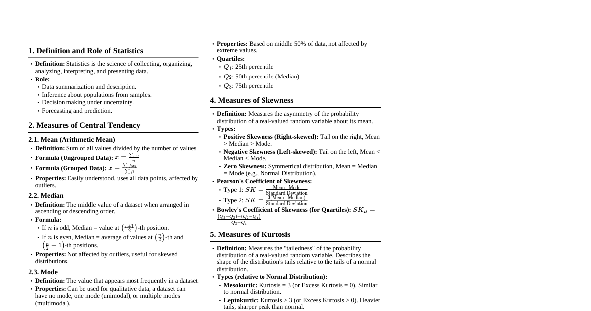
1. Fundamental Concepts Statistics: The science of collecting, organizing, analyzing, interpreting, and presenting data. Data: Facts and statistics collected together for reference or analysis. Population: The entire group of individuals or objects under consideration in a statistical study. Sample: A subset of the population selected for study. Parameter: A numerical characteristic of a population (e.g., population mean $\mu$). Variable: A characteristic or attribute that can be measured or observed. Types of Variables: Qualitative (Categorical): Describes non-numeric characteristics (e.g., gender, color). Quantitative (Numeric): Describes numeric characteristics (e.g., height, age). Discrete: Can only take specific, distinct values (e.g., number of children). Continuous: Can take any value within a given range (e.g., temperature). Types of Data: Primary Data: Collected directly by the researcher for the specific purpose. Secondary Data: Data collected by someone else for other purposes, but used by the researcher. 2. Levels of Measurement (Scales) Nominal Data: Categories without any order (e.g., eye color). Ordinal Data: Categories with a meaningful order, but unequal intervals (e.g., satisfaction ratings: low, medium, high). Interval Data: Ordered data with equal intervals between values, but no true zero point (e.g., temperature in Celsius/Fahrenheit). Ratio Data: Ordered data with equal intervals and a true zero point, allowing for ratios (e.g., height, weight). 3. Data Organization & Visualization Frequency Distribution: A table that displays the frequency of various outcomes in a sample. Ungrouped: For small datasets or discrete variables. Grouped: For large datasets or continuous variables, data is grouped into classes/intervals. Relative Frequency Distribution: Shows the proportion of observations within each category or class. Formula: $\text{Relative Frequency} = \frac{\text{Frequency}}{\text{Total Observations}}$ Cumulative Frequency Distribution: Shows the total number or proportion of observations that fall below the upper boundary of each category or class. Graphical Representation of Data: Visual displays of data. Types: Bar charts, Histograms, Pie charts, Line graphs, Scatter plots, Box plots, Stem-and-leaf plots. General Rules: Clear title, labeled axes, appropriate scale, legend (if needed), source. Box and Whisker Plot: Displays the five-number summary (minimum, Q1, median, Q3, maximum). Effective for showing distribution shape and outliers. Stem and Leaf Plot: Organizes data by splitting each data point into a "stem" (first digit(s)) and a "leaf" (last digit). Useful for showing distribution shape and individual data points. 4. Measures of Central Tendency Mean ($\bar{x}$ or $\mu$): The arithmetic average of a dataset. Sum of values divided by the number of values. $\bar{x} = \frac{\sum x_i}{n}$ Median: The middle value in an ordered dataset. If $n$ is even, it's the average of the two middle values. Mode: The value that appears most frequently in a dataset. A dataset can have no mode, one mode (unimodal), or multiple modes (multimodal). 5. Measures of Position Quartiles: Divide data into four equal parts (Q1, Q2=Median, Q3). $Q_1$: 25th percentile $Q_2$: 50th percentile (Median) $Q_3$: 75th percentile Deciles: Divide data into ten equal parts. $D_1$ is the 10th percentile, $D_9$ is the 90th percentile. Percentiles: Divide data into one hundred equal parts. The $P$-th percentile is the value below which $P$ percent of the observations fall. 6. Measures of Dispersion (Variability) Range: The difference between the maximum and minimum values in a dataset. $Range = Max - Min$. Variance ($\sigma^2$ or $s^2$): The average of the squared differences from the mean. Population Variance: $\sigma^2 = \frac{\sum (x_i - \mu)^2}{N}$ Sample Variance: $s^2 = \frac{\sum (x_i - \bar{x})^2}{n-1}$ Standard Deviation ($\sigma$ or $s$): The square root of the variance. It measures the typical distance of data points from the mean. Population Standard Deviation: $\sigma = \sqrt{\sigma^2}$ Sample Standard Deviation: $s = \sqrt{s^2}$ 7. Distribution Shape & Outliers Skewness: A measure of the asymmetry of the probability distribution of a real-valued random variable about its mean. Positive Skew (Right-skewed): Tail is longer on the right side; mean > median > mode. Negative Skew (Left-skewed): Tail is longer on the left side; mean Zero Skew: Symmetrical distribution; mean = median = mode. Kurtosis: A measure of the "tailedness" of the probability distribution of a real-valued random variable. Leptokurtic: High kurtosis, heavy tails, sharper peak than normal distribution. Mesokurtic: Medium kurtosis, similar to a normal distribution. Platykurtic: Low kurtosis, light tails, flatter peak than normal distribution. Outliers: Data points that significantly deviate from other observations. Definition: Typically defined as values outside $Q_1 - 1.5 \times IQR$ or $Q_3 + 1.5 \times IQR$, where $IQR = Q_3 - Q_1$. Causes: Measurement error, natural variation, data entry errors. Handling Outliers: Investigate, correct errors, remove (if justified), transform data, use robust statistical methods. Consequences: Can distort measures of central tendency (especially mean), inflate variance/standard deviation, affect model assumptions. 8. Regression & Correlation Regression: A statistical method used to describe the relationship between a dependent variable and one or more independent variables. Aims to predict the value of a dependent variable based on the value of an independent variable. Correlation: Measures the strength and direction of a linear relationship between two quantitative variables. Correlation Coefficient ($r$): Ranges from -1 to +1. $r=1$: Perfect positive linear relationship. $r=-1$: Perfect negative linear relationship. $r=0$: No linear relationship. 9. Probability Probability: The measure of the likelihood that an event will occur. $P(A) = \frac{\text{Number of favorable outcomes}}{\text{Total number of possible outcomes}}$. Ranges from 0 (impossible) to 1 (certain). 10. Short Questions & Key Concepts What Does Statistics Do? Provides tools to make sense of data, draw conclusions, and make informed decisions in the face of uncertainty. Why Do We Need Data? Data is the raw material for understanding phenomena, testing hypotheses, and solving problems in various fields. What is Data Visualization? The graphical representation of information and data to help users understand complex data or identify patterns. How to Organize Data? Through tables (frequency distributions), sorting, grouping, and preparing for analysis. Why is Data Analysis Important? It allows us to extract insights, identify trends, predict future outcomes, and support decision-making. Why Is Statistics Used in All Fields? Because data collection and analysis are crucial for research, decision-making, quality control, forecasting, and understanding variability in virtually every domain. Difference between structured, unstructured and semi-structured data: Structured: Highly organized data, typically in tabular format with predefined schemas (e.g., relational databases). Unstructured: Data without a predefined format or organization (e.g., text documents, images, audio). Semi-structured: Has some organizational properties, but not strictly rigid like structured data (e.g., XML, JSON files). Why are levels of measurement important? They determine which statistical analyses are appropriate for a given variable. Using the wrong level can lead to invalid conclusions. Measures of Central Tendency, Applications in Real Life: Mean (average income), Median (housing prices to avoid outlier distortion), Mode (most popular product size). Applications in Real Life: Quality control in manufacturing, medical research (drug efficacy), financial forecasting, public opinion polls, weather prediction.