Statistics Essentials

Cheatsheet Content

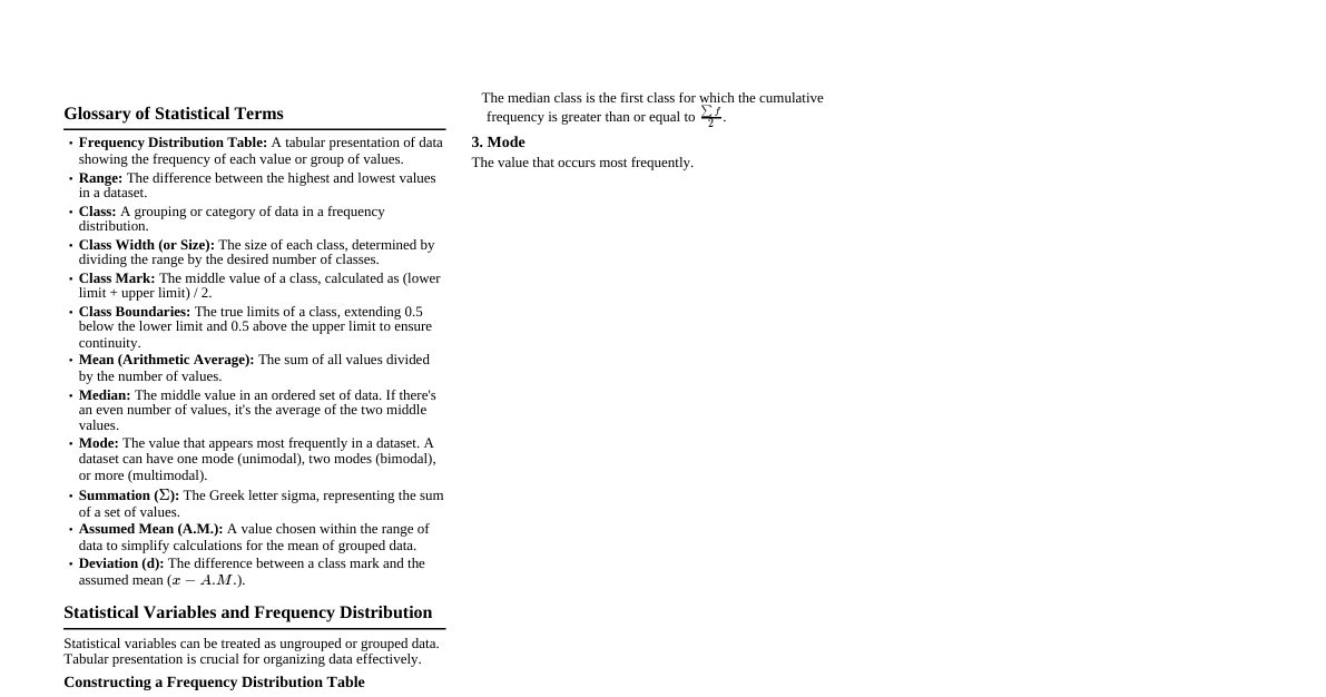
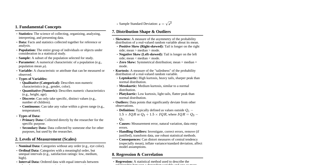
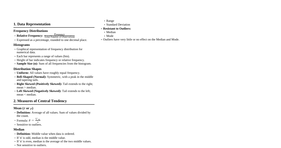
1. Definition and Role of Statistics Definition: Statistics is the science of collecting, organizing, analyzing, interpreting, and presenting data. Role: Data summarization and description. Inference about populations from samples. Decision making under uncertainty. Forecasting and prediction. 2. Measures of Central Tendency 2.1. Mean (Arithmetic Mean) Definition: Sum of all values divided by the number of values. Formula (Ungrouped Data): $\bar{x} = \frac{\sum x_i}{n}$ Formula (Grouped Data): $\bar{x} = \frac{\sum f_i x_i}{\sum f_i}$ Properties: Easily understood, uses all data points, affected by outliers. 2.2. Median Definition: The middle value of a dataset when arranged in ascending or descending order. Formula: If $n$ is odd, Median = value at $\left(\frac{n+1}{2}\right)$-th position. If $n$ is even, Median = average of values at $\left(\frac{n}{2}\right)$-th and $\left(\frac{n}{2}+1\right)$-th positions. Properties: Not affected by outliers, useful for skewed distributions. 2.3. Mode Definition: The value that appears most frequently in a dataset. Properties: Can be used for qualitative data, a dataset can have no mode, one mode (unimodal), or multiple modes (multimodal). 2.4. Geometric Mean (GM) Definition: The $n$-th root of the product of $n$ values. Useful for growth rates or ratios. Formula: $GM = \sqrt[n]{x_1 \cdot x_2 \cdot \ldots \cdot x_n}$ or $\log(GM) = \frac{1}{n} \sum \log(x_i)$ Properties: Sensitive to small values, requires all values to be positive. 2.5. Harmonic Mean (HM) Definition: The reciprocal of the arithmetic mean of the reciprocals of the values. Useful for rates and ratios (e.g., average speed). Formula: $HM = \frac{n}{\sum \frac{1}{x_i}}$ Properties: Heavily influenced by small values, requires all values to be positive. 2.6. Relationship between AM, GM, HM For positive datasets: $AM \ge GM \ge HM$ Equality holds if and only if all data points are identical. 2.7. Weighted Averages Definition: Each data point $x_i$ is assigned a weight $w_i$. Formula: $\bar{x}_w = \frac{\sum w_i x_i}{\sum w_i}$ Usage: Calculating GPA, portfolio returns, etc. 2.8. Group Averages (Combined Mean) Definition: Mean of combined groups. Formula: $\bar{x}_{combined} = \frac{n_1 \bar{x}_1 + n_2 \bar{x}_2 + \ldots + n_k \bar{x}_k}{n_1 + n_2 + \ldots + n_k}$ 3. Measures of Dispersion (Variability) 3.1. Range Definition: The difference between the maximum and minimum values in a dataset. Formula: Range = $X_{max} - X_{min}$ Properties: Simple to calculate, highly sensitive to outliers. 3.2. Variance Definition: The average of the squared differences from the mean. Measures how far each number in the set is from the mean. Sample Variance: $s^2 = \frac{\sum (x_i - \bar{x})^2}{n-1}$ Population Variance: $\sigma^2 = \frac{\sum (x_i - \mu)^2}{N}$ Properties: Units are squared, gives more weight to larger deviations. 3.3. Standard Deviation (SD) Definition: The square root of the variance. Provides a measure of dispersion in the original units of the data. Sample Standard Deviation: $s = \sqrt{\frac{\sum (x_i - \bar{x})^2}{n-1}}$ Population Standard Deviation: $\sigma = \sqrt{\frac{\sum (x_i - \mu)^2}{N}}$ Properties: Widely used, easy to interpret, sensitive to outliers. 3.4. Mean Absolute Deviation (MAD) Definition: The average of the absolute differences from the mean (or median). Formula: $MAD = \frac{\sum |x_i - \bar{x}|}{n}$ Properties: Less sensitive to outliers than variance/SD, but mathematically less tractable. 3.5. Quartile Deviation (Semi-Interquartile Range) Definition: Half the difference between the third and first quartiles. Formula: $QD = \frac{Q_3 - Q_1}{2}$ Properties: Based on middle 50% of data, not affected by extreme values. Quartiles: $Q_1$: 25th percentile $Q_2$: 50th percentile (Median) $Q_3$: 75th percentile 4. Measures of Skewness Definition: Measures the asymmetry of the probability distribution of a real-valued random variable about its mean. Types: Positive Skewness (Right-skewed): Tail on the right, Mean > Median > Mode. Negative Skewness (Left-skewed): Tail on the left, Mean Zero Skewness: Symmetrical distribution, Mean = Median = Mode (e.g., Normal Distribution). Pearson's Coefficient of Skewness: Type 1: $SK = \frac{\text{Mean} - \text{Mode}}{\text{Standard Deviation}}$ Type 2: $SK = \frac{3(\text{Mean} - \text{Median})}{\text{Standard Deviation}}$ Bowley's Coefficient of Skewness (for Quartiles): $SK_B = \frac{(Q_3 - Q_2) - (Q_2 - Q_1)}{Q_3 - Q_1}$ 5. Measures of Kurtosis Definition: Measures the "tailedness" of the probability distribution of a real-valued random variable. Describes the shape of the distribution's tails relative to the tails of a normal distribution. Types (relative to Normal Distribution): Mesokurtic: Kurtosis = 3 (or Excess Kurtosis = 0). Similar to normal distribution. Leptokurtic: Kurtosis > 3 (or Excess Kurtosis > 0). Heavier tails, sharper peak than normal. Platykurtic: Kurtosis Formula (Excess Kurtosis): $K = \frac{E[(X-\mu)^4]}{(\sigma^2)^2} - 3$ 6. Measures of Economic Inequality Definition: Quantifies the disparity in income, wealth, or other economic metrics among individuals or groups within a population. Common Measures: Gini Coefficient: Ranges from 0 (perfect equality) to 1 (perfect inequality). Calculated from the Lorenz curve (a graphical representation of income distribution). Formula often involves areas under the Lorenz curve: $G = \frac{A}{A+B}$ where A is area between line of equality and Lorenz curve, B is area below Lorenz curve. Lorenz Curve: Plots the cumulative share of total income (or wealth) held by the cumulative share of the population, ordered from poorest to richest. Palma Ratio: Ratio of the income share of the top 10% to the income share of the bottom 40%. Theil Index: A measure of entropy, sensitive to changes at the lower and upper ends of the distribution. Income Quintile Ratios: Ratios comparing the income shares of different quintiles (e.g., richest 20% vs. poorest 20%).