Programming & Data Structures
Shared 5/12/2026•0 views
### Time Complexity Measures how algorithm running time grows with input size ($n$), independent of hardware/language. * **Big-O Notation ($O$):** Upper bound (worst case). E.g., $O(1), O(\log n), O(n), O(n \log n), O(n^2)$. * **Omega Notation ($\Omega$):** Lower bound (best case). * **Theta Notation ($\Theta$):** Tight bound (average case). * **Dominant Term Rule:** Drop lower-order terms and constants. E.g., $O(3n^2 + 2n + 5) = O(n^2)$. #### Time Complexity Categories | Notation | Name | Example | |----------|-------------|------------------------------------------| | $O(1)$ | Constant | Array access, stack push/pop | | $O(\log n)$| Logarithmic | Binary search | | $O(n)$ | Linear | Linear search, single traversal | | $O(n \log n)$| Linearithmic| Merge sort, heap sort | | $O(n^2)$ | Quadratic | Bubble, selection, insertion sort | | $O(2^n)$ | Exponential | Recursive Fibonacci (naive) | ### Space Complexity Additional memory used by an algorithm beyond input. * **In-place algorithms:** $O(1)$ extra space (e.g., Bubble, Selection, Insertion, Heap, Quicksort with partitioning). * **Out-of-place algorithms:** $O(n)$ extra space (e.g., Merge Sort). ### Arrays * **1D Array:** Collection of same data type elements in contiguous memory. * **Access:** $O(1)$ (direct address calculation). * **Address of A[i]:** `Base_address(A) + (i * size_of_element)`. * **2D Array:** Array of arrays (matrix-like). * **Row-major order:** Elements of a row stored contiguously. * **Address of A[i][j]:** `Base_address(A) + ((i * C + j) * size_of_element)` (where C is number of columns). #### Array Operations & Complexities | Operation | Time (1D/2D) | Reason | |-----------------------|--------------------------|------------------------------------------| | Access/Update by index| $O(1)$ | Direct memory address calculation | | Search (unsorted) | $O(n)$ / $O(rows \times cols)$ | May need to scan all elements | | Search (sorted) | $O(\log n)$ | Binary search possible | | Insert at end | $O(1)$ | If space available | | Insert at beginning/middle | $O(n)$ | All subsequent elements must shift right | | Delete at end | $O(1)$ | Just decrement size | | Delete at beginning/middle | $O(n)$ | All subsequent elements must shift left | | Traverse | $O(n)$ / $O(rows \times cols)$ | Visit every element once | * **Arrays are fast at access, slow at structure changes.** ### Searching #### Linear Search * Checks each element from left to right. * Works on sorted and unsorted arrays. * **Complexity:** $O(n)$ for 1D, $O(m \times n)$ for 2D. * **Best Case:** $\Omega(1)$ (key at index 0). * **Average Case:** $\Theta(n/2) = \Theta(n)$ (key in middle). * **Worst Case:** $O(n)$ (key at last position or not present). * **Space:** $O(1)$. * **When to use:** Small, unsorted datasets, single searches. ``` LINEAR_SEARCH(A, n, key) for each index i from 0 to n-1 if arr[i] == key return i return -1 ``` #### Binary Search * Repeatedly splits search space in half by comparing with the middle element. * Requires a **sorted array**. * **Complexity:** $O(\log n)$. * **Best Case:** $\Omega(1)$ (key at first mid). * **Average Case:** $\Theta(\log n)$. * **Worst Case:** $O(\log n)$ (key at leaf or absent). * **Space:** $O(1)$ iterative; $O(\log n)$ recursive (call stack depth). * **When to use:** Large sorted datasets, repeated searches. ``` BINARY_SEARCH(A, n, key) low ← 0 high ← n - 1 while low ≤ high do mid ← floor((low + high) / 2) if A[mid] = key then return mid else if A[mid] ### Sorting #### Bubble Sort * Compares adjacent elements and swaps them if they are in the wrong order. * Largest element "bubbles" to the end with each pass. * **Complexity:** * **Worst/Average Case:** $O(n^2)$ (array sorted in reverse/random). * **Best Case:** $\Omega(n)$ (array already sorted). * **Space:** $O(1)$ (in-place). * **Stable:** Yes. ``` BUBBLE_SORT(A, n) for i ← 0 to n - 1 do swapped ← false for j ← 0 to n - i - 2 do if A[j] > A[j + 1] then swap A[j] and A[j + 1] swapped ← true if swapped = false then break ``` #### Selection Sort * Finds the minimum (or maximum) element from the unsorted portion and swaps it with the first element of the unsorted portion. * **Complexity:** * **Worst/Average/Best Case:** $\Theta(n^2)$ (always performs $n^2$ comparisons). * **Space:** $O(1)$ (in-place). * **Stable:** No. ``` SELECTION_SORT(A, n) for i ← 0 to n - 2 do min_index ← i for j ← i + 1 to n - 1 do if A[j] key do A[j + 1] ← A[j] j ← j - 1 A[j + 1] ← key ``` #### Merge Sort * **Divide and Conquer:** Divides array into two halves, recursively sorts them, then merges the sorted halves. * **Complexity:** $\Theta(n \log n)$ (best, average, worst case). * **Dividing:** $\log n$. * **Merging:** $O(n)$ per level. * **Space:** $O(n)$ (new space created). * **Stable:** Yes. ``` MERGE_SORT(A) if left 0 do COUNTING_SORT(A, n, exp) // Counting Sort adapted for specific digit exp ← exp × 10 COUNTING_SORT(A, n, exp) // (Modified for Radix Sort) create array output[0 … n-1] create array count[0 … 9] initialized to 0 for i ← 0 to n-1 do digit ← (A[i] / exp) % 10 count[digit] ← count[digit] + 1 for i ← 1 to 9 do count[i] ← count[i] + count[i-1] for i ← n-1 down to 0 do digit ← (A[i] / exp) % 10 output[count[digit] - 1] ← A[i] count[digit] ← count[digit] - 1 for i ← 0 to n-1 do A[i] ← output[i] ``` ### Sort Algorithms Compared | Algorithm | Best | Average | Worst | Space | Stable | In-place | |---------------|---------------|---------------|---------------|-------------|--------|----------| | Bubble Sort | $\Omega(n)$ | $\Theta(n^2)$ | $O(n^2)$ | $O(1)$ | Yes | Yes | | Selection Sort| $\Omega(n^2)$ | $\Theta(n^2)$ | $O(n^2)$ | $O(1)$ | No | Yes | | Insertion Sort| $\Omega(n)$ | $\Theta(n^2)$ | $O(n^2)$ | $O(1)$ | Yes | Yes | | Merge Sort | $\Omega(n \log n)$| $\Theta(n \log n)$| $O(n \log n)$ | $O(n)$ | Yes | No | | Quick Sort | $\Omega(n \log n)$| $\Theta(n \log n)$| $O(n^2)$ | $O(\log n)$ | No | Yes | | Counting Sort | $\Omega(n+k)$ | $\Theta(n+k)$ | $O(n+k)$ | $O(n+k)$ | Yes | No | | Radix Sort | $\Omega(d(n+k))$| $\Theta(d(n+k))$| $O(d(n+k))$ | $O(d(n+k))$ | Yes | No | | Heap Sort | $\Omega(n \log n)$| $\Theta(n \log n)$| $O(n \log n)$ | $O(1)$ | No | Yes | ### Recursion * **Base Case:** Condition when the algorithm should stop (boundary of data or end of structure). * **Recursive Case:** Condition when the algorithm continues calling itself on a smaller sub-scope. * **Time Complexity:** Number of recursive calls. * **Space Complexity:** Depth of the recursion stack/tree. * **Insight:** Carry over a previously found solution forward. ### Abstract Data Types (ADT) * Language-independent model separating *what* a data structure does from *how* it does it. * Client sees interface, implementer owns internals. * Stack and Queue are ADTs, implementable by arrays or linked lists. ### Stack * **Principle:** LIFO (Last In, First Out). * **Key Invariant:** All insertions/deletions happen only at the `TOP` (tracked by `Top` pointer). `Top` starts at -1 (empty stack). #### Stack Operations | Operation | Description | Time | |----------------|-----------------------|------| | `push(x)` | Insert at top | $O(1)$ | | `pop()` | Remove from top | $O(1)$ | | `peek()/top()` | View top without removing | $O(1)$ | | `isEmpty()/isFull()` | Boundary checks | $O(1)$ | #### Push Operation 1. Check if stack is full (`isFull()`). 2. If full, report Overflow error. 3. If not full, move `TOP` pointer to next available position (`TOP = TOP + 1`). 4. Insert new data element at `S[TOP]`. ``` if(Top == C - 1) // C is stack capacity "stack is full"; else Top = Top + 1; S[Top] = x; ``` #### Pop Operation 1. Check if stack is empty (`isEmpty()`). 2. If empty, report Underflow error. 3. If not empty, assign element at `TOP` to a variable (`y = S[Top]`). 4. Move `TOP` pointer to previous location (`Top = Top - 1`). 5. Return the value `y`. ``` if(Top == -1) "stack is empty"; else int y; y = S[Top]; Top = Top - 1; return y; ``` #### Applications of Stack * Function Call Management (Call Stack). * Undo/Redo in Text Editors. * Parsing (compilers). * Browser History. * Balanced Parentheses Check. * Infix to Postfix/Prefix conversion and evaluation. ### Infix to Postfix Conversion * **Operands:** Go directly to output. * **Operators:** Held on a stack, released based on precedence and associativity. * `precedence(top) > precedence(incoming)`: Pop to output, then push incoming. * `equal precedence AND left-associative`: Pop to output, then push incoming. * `equal precedence AND right-associative` (e.g., `^`): Push directly. * **End of expression:** Flush remaining operators to output. * **Examples:** * `a+b*c` $\rightarrow$ `abc*+` (multiplication has higher precedence). * `a*b+c` $\rightarrow$ `ab*c+` (higher precedence pops first). * `a-b-c` $\rightarrow$ `ab-c-` (left-associative: pop first minus). * `a^b^c` $\rightarrow$ `abc^^` (right-associative: do not pop). ### Postfix Evaluation * **Scan left to right.** * **Operand:** Push onto stack. * **Operator:** Pop two operands (`op2` first, `op1` second), compute `op1 operator op2`, push result onto stack. * **Final result:** Single remaining element on stack. * **Important:** First popped = `op2`, Second popped = `op1` (order matters for subtraction and division). ### Queue * **Principle:** FIFO (First In, First Out). * **Key Invariant:** Insertion at `REAR`, deletion at `FRONT`. Both `F` and `R` start at -1; `F` moves to 0 on the first enqueue. #### Queue Operations | Operation | Description | Time | |----------------|-----------------------|------| | `enqueue(x)` | Insert at rear | $O(1)$ | | `dequeue()` | Remove from front | $O(1)$ | | `peek()` | View front | $O(1)$ | | `isEmpty()/isFull()` | Boundary checks | $O(1)$ | #### Enqueue Operation 1. Check if queue is full (`isFull()`). 2. If full, report Overflow error. 3. If not full, move `REAR` pointer to next available position. If `F == -1`, set `F = 0` (first enqueue). 4. Insert new data element at `Q[R]`. ``` if(R == C - 1) // C is queue capacity "queue is full"; if F == -1 then F ← 0 // first enqueue R = R + 1; Q[R] = x; ``` #### Dequeue Operation 1. Check if queue is empty (`isEmpty()`). 2. If empty, report Underflow error. 3. If not empty, assign element at `FRONT` to a variable (`y = Q[F]`). 4. Move `FRONT` pointer to next available position. If `F == R`, reset `F` and `R` to -1 (queue now empty). 5. Return the value `y`. * **Key Point:** First retrieve the data, then increment the `FRONT` pointer. ``` if(F == -1) "queue is empty"; int y; y = Q[F]; if(F == R) Reset F and R → -1; else F = F + 1; return y; ``` #### Applications of Queue * CPU Scheduling. * Handling website traffic. * Managing customer service lines. * Traffic management systems. * Network packet transmission. * Implementing algorithms like Breadth-First Search (BFS). ### Circular Queue * **Problem:** Linear queue wastes unused space after multiple dequeue operations. * **Fix:** Treat array as circular. Replace pointer movement with modular arithmetic: `(pointer + 1) % size`. `REAR` wraps back to index 0 after reaching last slot. * **Key Invariant:** All insertions at `REAR`, all deletions at `FRONT`; both pointers always move as `(pointer + 1) % size`. #### Circular Queue States & Conditions | State | Condition | |-------|-----------------------------| | Empty | `F == -1` | | Full | `(R + 1) % size == F` | | Size | `(R - F + C) % C` (C=capacity) | #### Enqueue (Circular) ``` ENQUEUE(x) IF ( (rear + 1) MOD size = front ) THEN PRINT "Queue is Full" RETURN END IF IF ( front = -1 ) THEN front ← 0 rear ← 0 ELSE rear ← (rear + 1) MOD size END IF queue[rear] ← x END ENQUEUE ``` #### Dequeue (Circular) ``` DEQUEUE() IF ( front = -1 ) THEN PRINT "Queue is Empty" RETURN END IF element ← array[front] IF ( front = rear ) THEN front ← -1 rear ← -1 ELSE front ← (front + 1) MOD size END IF RETURN element ``` ### Linked List #### Singly Linked List (SLL) * **Nodes:** Stored in non-contiguous memory; each node holds `data` and a `next` pointer. * `head` points to the first node; last node's `next = NULL`. * **Key Invariant:** Starting from `head`, repeatedly following `next` must reach every node exactly once and eventually reach `NULL`. ##### SLL Operations & Complexities | Operation | Time | Reason | |-----------------------|------|------------------------| | Insert at beginning | $O(1)$ | No traversal needed | | Insert at end | $O(n)$ | Must traverse to last node | | Insert at position | $O(n)$ | Must traverse to `pos-1` | | Delete at beginning | $O(1)$ | Just move `head` | | Delete at end | $O(n)$ | Must find second-to-last | | Delete at position | $O(n)$ | Must traverse | | Search | $O(n)$ | Sequential access only | ##### SLL Insertion (Pseudocode) * **Case 1: Insert at beginning** ``` first→next = head head = first ``` * **Case 2: Insert at end** ``` temp = head while(temp→next != NULL) temp = temp→next temp→next = last ``` * **Case 3: Insert at specific position** ``` temp = head index = 0 while(temp→next != NULL and index ### Tree #### Tree Terminology * **Root:** Node with no parent. * **Leaf:** Node with no children (external node). * **Internal Node:** Node with at least one child. * **Depth of a Node:** Number of ancestors (root has depth 0). * **Height of Tree:** Maximum depth of any node. * **Subtree:** A node and all its descendants. * **Size:** Total number of nodes. * **Key Property:** A tree with $N$ nodes has exactly $N-1$ edges. #### Binary Tree * Each node has at most 2 children (left and right). * **Array representation:** * `rank(root) = 1` * `left child (of parent at i) = 2 * i` * `right child (of parent at i) = 2 * i + 1` * `parent (of node at i) = floor(i/2)` #### Tree Traversals * **Key fact:** For BST, Inorder traversal always yields elements in ascending sorted order. | Traversal | Order | Root Order | Application | |-----------|---------------------|-------------|--------------------------| | Preorder | Root $\rightarrow$ Left $\rightarrow$ Right | Root first | Print structured document | | Inorder | Left $\rightarrow$ Root $\rightarrow$ Right | Root middle | Sorted output from BST | | Postorder | Left $\rightarrow$ Right $\rightarrow$ Root | Root last | Compute directory sizes | ### Binary Search Tree (BST) * **Key Invariant:** Left subtree values $\le$ node value $\le$ right subtree values (for every node). #### BST Search * **Best Case:** $\Omega(1)$ (key is root). * **Average Case:** $\Theta(\log n)$ (balanced tree, height = $\log n$). * **Worst Case:** $O(n)$ (skewed/unbalanced tree, height = $n$). #### BST Insertion * Follow BST property to find correct `NULL` position, insert there. #### BST Deletion (3 cases) 1. **Leaf node:** Simply delete, point parent to `NULL`. 2. **One child:** Link parent to child, replace node with its child. 3. **Two children:** Replace with inorder predecessor (max of left subtree) OR inorder successor (min of right subtree), then delete that replacement node. ### AVL Tree * **Problem with BST:** Insertion in sorted order produces a skewed tree, degrading operations to $O(n)$, motivating balanced BSTs. * **AVL = BST + Self-Balancing via Balance Factor.** * **Balance Factor (BF) of a node:** `height(left subtree) - height(right subtree)`. * **Key Invariant:** `BF ∈ {-1, 0, +1}` for every node at all times. * **Rotations:** When BF goes outside this range after insertion/deletion, rotations restore balance. * **Height:** Always guaranteed to be $\log n$. #### Rotations (Four cases) * **LL case (Left Left):** Left child in left subtree $\rightarrow$ Single right rotation. * **RR case (Right Right):** Right child in right subtree $\rightarrow$ Single left rotation. * **LR case (Left Right):** Left child in right subtree $\rightarrow$ Left rotation on child, then right rotation on grandparent. * **RL case (Right Left):** Right child in left subtree $\rightarrow$ Right rotation on child, then left rotation on grandparent. * **Complexity (Insertion and Deletion):** $O(\log n)$ due to height guarantee. * **Limitation:** Write-heavy workloads cause frequent rotations $\rightarrow$ overhead grows $\rightarrow$ Red-Black Tree is often preferred. ### Red-Black Tree #### Properties 1. Every node is Red or Black. 2. Root is always Black. 3. All `NULL` leaves are considered Black. 4. Red nodes cannot have Red children (no two consecutive Reds). 5. Every path from a node to any descendant `NULL` leaf has the same number of Black nodes (Black Height). * **Key Invariant:** Left ### AVL vs RBT | Property | AVL Tree | Red-Black Tree | |-------------------|--------------------------|-------------------------------| | Balance | Strict (BF $\in$ {-1, 0, +1}) | Approximate (height $\le 2 \cdot \log n$) | | Search | Faster (shorter height) | Slightly slower | | Insertion rotations| More frequent | $\le 2$ per insertion | | Deletion rotations| More frequent | $\le 3$ per deletion | | Best use case | Read-heavy systems involving search | Read-write balanced systems | ### Heap #### Heap Properties * **Shape property:** Complete binary tree (all levels full except possibly last, filled left to right). * **Heap property:** Max-Heap – parent $\ge$ children; Min-Heap – parent $\le$ children. * **Key Invariant (Max-Heap):** Parent $\ge$ children AND tree is always complete. * **Root:** Always the max (Max-Heap) or min (Min-Heap). * **Height:** Always $\log_2 n$ $\rightarrow$ all operations $O(\log n)$. * **Important:** A heap is NOT a BST – no left/right ordering relationship. * **Array representation:** index 1 is root; left child = $2 \cdot i$; right child = $2 \cdot i + 1$; parent = $\text{floor}(i/2)$. #### Heapify * **Heapify Down (Sift Down):** Used after deletion (always at root, replaced with last element). * Node at root is too small (Max-Heap). * Find largest among node and its direct children; swap if needed; recurse on swapped position. * Stops when node $\ge$ both children or node is a leaf. * **Time:** $O(\log n)$ – works along one root-to-leaf path. * **Heapify Up (Sift Up):** Used after insertion. * Newly inserted node may be too large (Max-Heap). * Compare with parent; swap if violation; repeat upward. * **Time:** $O(\log n)$. * **MAX_HEAPIFY assumption:** When called on node $i$, both subtrees rooted at left($i$) and right($i$) must already be valid heaps. #### Heap Operations | Operation | Time | Method | |----------------|-------------|--------------------------| | Access max/min | $O(1)$ | Read root | | Insert | $O(\log n)$ | Append at end, Heapify Up| | Delete root | $O(\log n)$ | Replace with last element, Heapify Down | | Build Heap | $O(n)$ | Bottom-up MAX_HEAPIFY | | Heap Sort | $O(n \log n)$ | Build + repeated extraction | #### Build Heap * Start at the first non-leaf node (index $n//2$), call `MAX_HEAPIFY` backward to index 1. * **Time:** $O(n)$ – not $O(n \log n)$, because most nodes are near the leaves and do little work. * **Intuition:** leaves ($\approx n/2$) do no work; nodes one level up ($\approx n/4$) do at most 1 swap; etc. #### Heap Sort * **Algorithm:** Repeatedly swap root with last element, reduce heap size, call `MAX_HEAPIFY` on root. * **Max-Heap:** $\rightarrow$ ascending order output. * **Min-Heap:** $\rightarrow$ descending order output. * **Time:** $O(n \log n)$. * **Space:** $O(1)$ (in-place). * **Not stable:** Equal elements may be reordered. * Worse cache performance than Quicksort in practice despite same asymptotic bound. * **Best suited when repeated max/min search is the priority.** #### Heap vs BST vs AVL/RBT | Property | Heap | BST | AVL/RBT | |-------------------|-------------|---------------|-------------| | Find min/max | $O(1)$ | $O(n)$/$O(\log n)$ | $O(\log n)$ | | Insert | $O(\log n)$ | $O(n)$ worst | $O(\log n)$ | | Delete min/max | $O(\log n)$ | $O(n)$ worst | $O(\log n)$ | | Search arbitrary | $O(n)$ | $O(n)$ worst | $O(\log n)$ | ### Graph #### Graph Terminology * **Graph G = (V, E):** Set of vertices (V) and edges (E). * **Adjacent:** Two vertices directly connected by an edge. * **Degree (undirected):** Number of edges at a vertex. **Key Invariant:** Sum of all degrees = $2|E|$. * **In-degree / Out-degree (directed):** Edges pointing in / out. **Key Invariant:** Sum of in-degrees = sum of out-degrees = $|E|$. * **Path:** Sequence of vertices connected by edges; length = number of edges. * **Simple Path:** No repeated vertices. * **Cycle:** Path that starts and ends at the same vertex. * **Connected:** Path exists between every pair of vertices. * **DAG (Directed Acyclic Graph):** Directed, no cycles; at least one source (in-degree 0) and one sink (out-degree 0). #### Graph Types | Type | Key Property | |--------------------|--------------------------------------------------| | Undirected | (A,B) = (B,A), symmetric edges | | Directed | (A,B) $\neq$ (B,A), non-symmetric edges | | Weighted | Edges carry a cost value | | Complete ($K_n$) | Every pair connected; $n(n-1)/2$ edges; every vertex has degree $n-1$ | | Regular | All vertices have the same degree | | Disconnected | Some vertices unreachable from others | | Acyclic undirected | Is a tree | | DAG | Directed, no cycles; supports topological sort | #### Graph Representation | | Edge List | Adjacency Matrix | Adjacency List | |------------|----------------|------------------|--------------------| | Space | $O(E)$ | $O(V^2)$ | $O(V+E)$ | | Check edge (u,v) | $O(E)$ | $O(1)$ | $O(\text{degree}(u))$ | | All neighbors of v | $O(E)$ | $O(V)$ | $O(\text{degree}(v))$ | | Iterate all edges | $O(E)$ | $O(V^2)$ | $O(V+E)$ | | Best for | Kruskal's | Dense graphs | Sparse graphs, BFS, DFS | * **Rule of thumb:** * **Adjacency list:** For sparse graphs. * **Adjacency matrix:** For dense graphs or when $O(1)$ edge lookup is needed. * **Edge list:** For algorithms that iterate all edges. ### Breadth First Search (BFS) * **Data structure:** Queue. * **Strategy:** Level-by-level; all vertices at distance $k$ processed before any at distance $k+1$. * **Key Invariant:** BFS always finds the minimum-edge-count (hop) path – unweighted graphs only. * **Vertex states:** Undiscovered $\rightarrow$ Discovered (in queue) $\rightarrow$ Processed (dequeued, in visited set). #### BFS Process 1. Mark all vertices undiscovered; enqueue source. 2. While queue not empty: * Dequeue $u$. * For each undiscovered neighbor $v$: * Mark $v$ discovered, enqueue $v$. * Mark $u$ as processed/visited. ``` BFS(G, s): for each vertex u in G.V − {s}: u.discovered = FALSE s.discovered = TRUE Q = empty queue ENQUEUE(Q, s) while Q is not empty: u = DEQUEUE(Q) for each v in Adj[u]: if v.discovered == FALSE: v.discovered = TRUE ENQUEUE(Q, v) u.visited = TRUE ``` #### BFS Properties * **Complexity:** Time $O(V+E)$; Space $O(V)$. * **Extensions:** Distance array $d[v]$ (hops from source), Predecessor array $\pi[v]$, BFS tree. * **Applications:** Shortest path (unweighted), web crawlers, social network degrees of separation, cycle detection. * **Limitation:** Does not handle edge weights; must re-run from each unvisited vertex for disconnected graphs. ### Depth First Search (DFS) * **Data structure:** Recursion (implicit call stack) or explicit Stack. * **Strategy:** Explore one branch as deep as possible before backtracking. * **Key Invariant:** When DFS finishes a vertex, every vertex reachable from it has already been discovered. * **Vertex states:** Undiscovered $\rightarrow$ Discovered (in stack) $\rightarrow$ Visited/Processed (popped, in visited set). #### DFS Process 1. Mark all vertices undiscovered; start at any vertex, mark discovered. 2. For all undiscovered vertices in graph: * Recursively visit unvisited neighbors, going deep along a single path. * If no unvisited neighbors, mark vertex as processed/visited. * Backtrack to previous vertex to explore remaining branches. ``` DFS(G, s): for each vertex u in G.V − {s}: u.discovered = FALSE u.visited = FALSE for each vertex u in G.V − {s}: if u.discovered == FALSE: DFS_VISIT(u) DFS_VISIT(u): u.discovered = TRUE for each v in Adj[u]: if v.discovered == FALSE: DFS_VISIT(v) u.visited = TRUE ``` #### DFS Properties * **Complexity:** Time $O(V+E)$; Space $O(V)$. * **Extensions:** Timestamps ($d[v]$ discovery, $f[v]$ finish), Edge Classification (directed graphs). * **Key fact:** A back edge found during DFS means a cycle exists in the graph. * **Applications:** Cycle detection, topological sort (reverse finish order on DAG), dependency resolution, maze solving, connected components. * **Limitation:** Does not guarantee shortest path; recursion upper bound. ### BFS vs DFS | | BFS | DFS | |------------|------------------------|---------------------------| | Structure | Queue (FIFO) | Stack / Recursion (LIFO) | | Order | Level by level | Deep first | | Shortest path | Yes (unweighted only) | Not guaranteed | | Timestamps | No | Yes | | Topological sort | No | Yes | | Cycle detection | Yes | Yes | | Best for | Shortest hops, level structure | Structural analysis, ordering | ### Minimum Spanning Tree (MST) #### Definitions * **Spanning Tree:** A subgraph that is a tree (connected, acyclic) and includes all $V$ vertices; has exactly $V-1$ edges. * Complete graphs have $n^{n-2}$ possible spanning trees. * **Minimum Spanning Tree (MST):** The spanning tree with the minimum total edge weight. * MST is only meaningful for connected, weighted, undirected graphs. * MST is NOT the shortest path between vertices. * If edge weights are distinct, MST will be unique. * **Greedy Algorithm:** Makes the optimal choice at each step based on information available only at the present. #### Prim’s Algorithm * **Strategy:** Grow the MST one vertex at a time; always add the minimum-weight edge connecting the current tree to a new vertex (or the visited side of the cut to the unvisited side of the cut). * **Uses:** Adjacency List and a priority queue. * **Time:** $O(E \log V)$ with a binary heap, $O(V^2)$ with arrays. * **Works well on dense graphs.** ``` PRIM_OPTIMIZED(G, w, s): for each vertex u in G.V: key[u] = ∞ π[u] = NIL key[s] = 0 Q = G.V // Q is a min-priority queue while Q is not empty: u = EXTRACT_MIN(Q) for each v in Adj[u]: if v ∈ Q and w(u,v) ### Dijkstra's Algorithm * **Problem:** Single-source shortest-path – find the cheapest path from one source vertex to all others on a **weighted graph**. * **Strategy:** Greedy – always finalize the unvisited vertex with the smallest known distance from source. * **Key Invariant:** Once a vertex $u$ is finalized, its shortest distance $u.d$ will never decrease again. * **Relaxation:** * For neighbor $v$ of $u$: if $v.d > u.d + w(u,v)$ $\rightarrow$ update $v.d = u.d + w(u,v)$, set $v.\pi = u$. * This is the core operation that updates shortest paths through $u$. #### Dijkstra's Algorithm - Pseudocode ``` DIJKSTRA(G, s): for each vertex v in G.V: v.d = ∞ // Initialize distances (0 for source, infinite for all others) v.π = NIL // Predecessor s.d = 0 S = {} // Empty set of finalized vertices Q = G.V // Min-priority queue (unvisited vertices queued by distance) while Q is not empty: u = EXTRACT_MIN(Q) // Process the closest vertex from the source S = S ∪ {u} for each v in Adj[u]: RELAX(u, v, w) // Apply relaxation on every neighbor // Reorganize Q with new distances (implicit in priority queue implementation) ``` #### Dijkstra's Algorithm - Properties * **Complexity:** $O(V^2)$ with simple array; $O(E \log V)$ with priority queue (binary heap). * **Critical limitation:** Only correct when all edge weights are **non-negative**. * Negative edges cause greedy finalization to produce wrong answers. * Negative weight cycles make shortest path $-\infty$; Dijkstra's cannot detect this. * **Applications:** GPS navigation, OSPF routing protocol, flight route optimization, robotics motion planning. ### Hashing * **Core idea:** Map keys to array indices using a hash function $\rightarrow$ average $O(1)$ search, insert, delete. * **Hash function example:** `h(key) = key mod size_of_table`. * **Collision:** When `h(key₁) = h(key₂)` but `key₁ ≠ key₂`. * **Collision Resolution Techniques:** | Method | Formula | Behavior | |-------------------|------------------------------|---------------------------------| | Linear Probing | `(h(key) + i) mod size` | Sequential scan; primary clustering | | Quadratic Probing | `(h(key) + i²) mod size` | Reduces clustering; secondary clustering | | Double Hashing | `(h1(key) + i·h2(key)) mod size` | Best distribution; most computation | * **Double hashing functions:** * `h1(key) = key mod size` * `h2(key) = 1 + (key mod (size - 1))` #### Hash Tables vs Other Data Structures | Structure / Algorithm | Search | Insert | Delete | Ordered? | Worst case search | |-----------------------|-------------|-------------|-------------|----------|-------------------| | Hash table | $O(1)$ avg | $O(1)$ avg | $O(1)$ avg | No | $O(n)$ | | AVL/RBT | $O(\log n)$ | $O(\log n)$ | $O(\log n)$ | Yes | $O(\log n)$ | | Heap | $O(n)$ | $O(\log n)$ | $O(\log n)$ | No | $O(n)$ | | Sorted array | $O(\log n)$ | $O(n)$ | $O(n)$ | Yes | $O(\log n)$ | * **Use hash tables when:** Fast average-case lookup matters and order is irrelevant. * **Do not use when:** Range queries needed, or sorted key order required. * **Worst case:** $O(n)$ – all keys collide to same index. * **Applications:** Python dictionaries, Java HashMaps, database exact-match indexing, caching, deduplication. ### A* Search * **Problem:** Single-source single-destination shortest path – faster than Dijkstra's by using domain knowledge (heuristic). * **Core idea:** Instead of just tracking actual cost from source ($g(u)$), also estimate remaining cost to goal ($h(u)$). * **Cost function:** $f(u) = g(u) + h(u)$ * $g(u)$ = actual cost of best-known path from source to $u$. * $h(u)$ = heuristic estimate of cost from $u$ to goal. * $f(u)$ = total estimated cost of cheapest path through $u$. #### Heuristic * **Heuristic must be admissible:** $h(u) \le h^*(u)$ (never overestimates the true cost). * Overestimating can cause A* to skip the actual shortest path. * $h(u) = 0$ for all $u$ is valid but reduces A* exactly to Dijkstra’s. * **Common heuristics:** * **Manhattan distance (grid, 4-directional movement):** $|u.x - goal.x| + |u.y - goal.y|$ * **Euclidean distance (free/diagonal movement):** $\sqrt{((u.x - goal.x)^2 + (u.y - goal.y)^2)}$ * Both admissible because they ignore obstacles (true path is always at least as long). #### A* Search - Process * Maintain a priority queue ordered by $f(u)$. * Extract minimum $f$, check if goal. * For each neighbor of extracted vertex: * Relax neighbors if $g(u) + w(u,v) ### Cross-Topic Summary | Structure / Algorithm | Search | Insert | Delete | Space | |-----------------------|-------------|-------------|-------------|-----------------| | Array (unsorted) | $O(n)$ | $O(1)$ | $O(n)$ | $O(n)$ | | Array (sorted) | $O(\log n)$ | $O(n)$ | $O(n)$ | $O(n)$ | | Stack / Queue | $O(1)$ top/front only | $O(1)$ | $O(1)$ | $O(n)$ | | SLL | $O(n)$ | $O(1)$ begin / $O(n)$ end | $O(1)$ begin / $O(n)$ end | $O(n)$ | | DLL (with tail) | $O(n)$ | $O(1)$ begin+end | $O(1)$ begin+end | $O(n)$ | | BST | $O(n)$ worst | $O(n)$ worst | $O(n)$ worst | $O(n)$ | | AVL Tree | $O(\log n)$ | $O(\log n)$ | $O(\log n)$ | $O(n)$ | | Red-Black Tree | $O(\log n)$ | $O(\log n)$ | $O(\log n)$ | $O(n)$ | | Heap (max/min) | $O(n)$ arbitrary | $O(\log n)$ | $O(\log n)$ root only | $O(n)$ | | Hash Table | $O(1)$ avg | $O(1)$ avg | $O(1)$ avg | $O(n)$ | | BFS / DFS | $O(V+E)$ | - | - | $O(V)$ | | Dijkstra's | $O(E \log V)$ | - | - | $O(V)$ | | Build Heap | - | $O(n)$ bulk | - | $O(n)$ | | Heap Sort | - | - | - | $O(1)$ in-place |