Numerical Linear Algebra

Cheatsheet Content

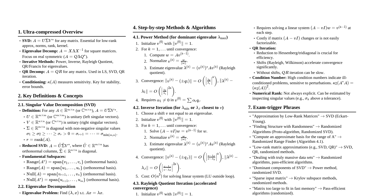
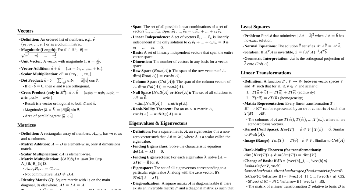
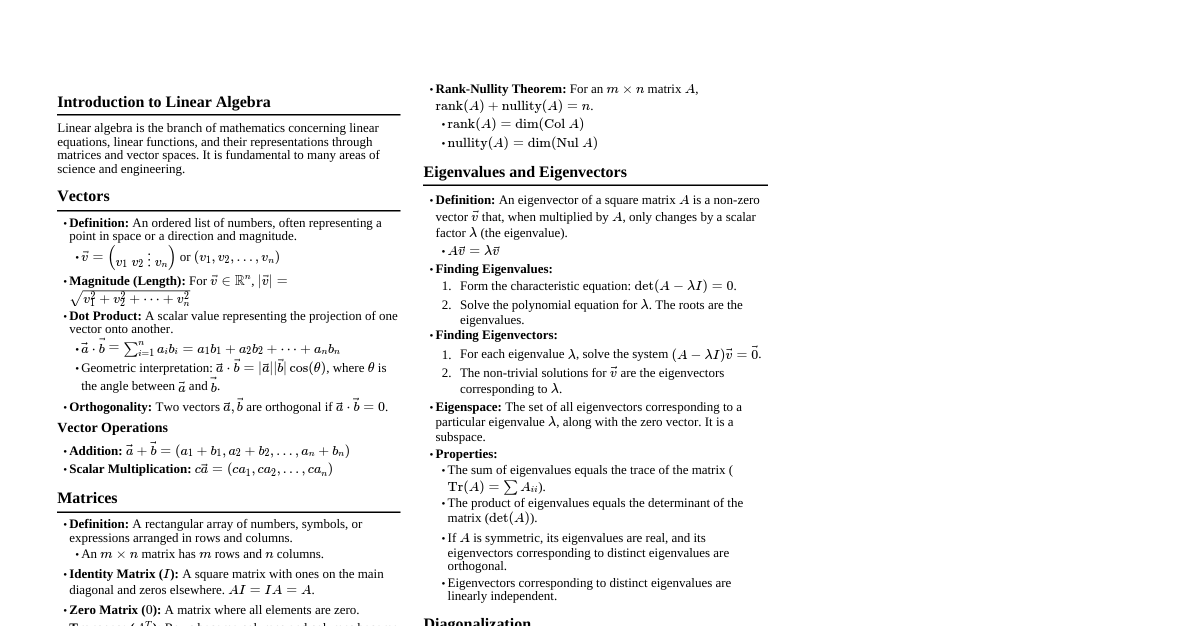
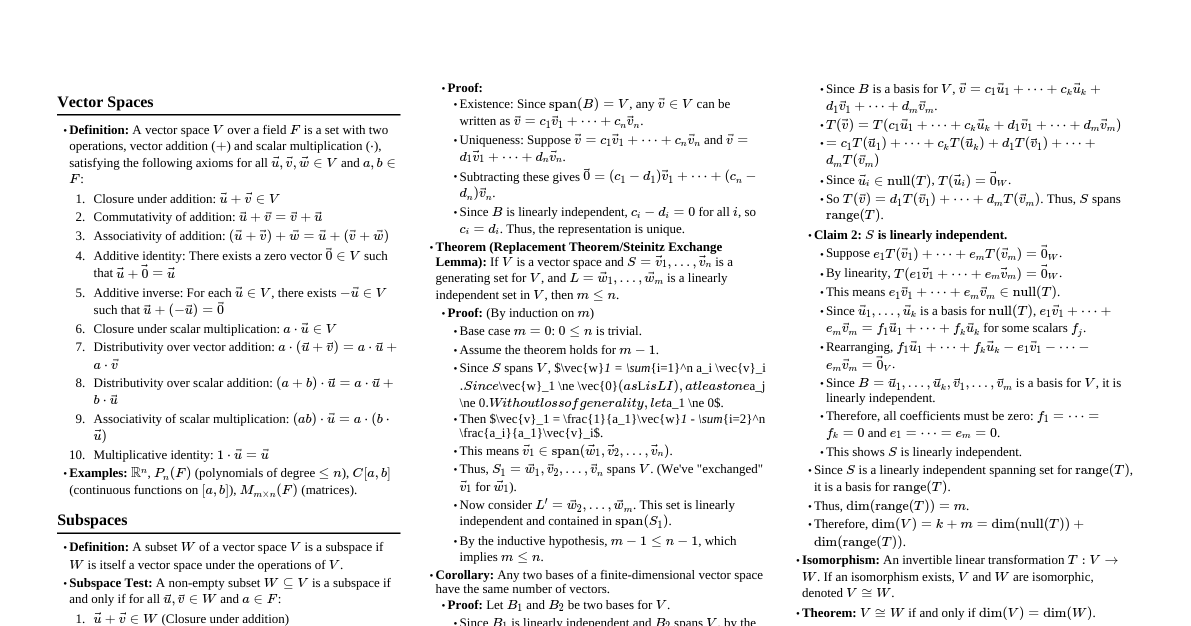
### Introduction This cheatsheet covers numerical methods for solving systems of linear equations, understanding their stability, and finding eigenvalues and eigenvectors. ### Norms Norms measure the "size" or "magnitude" of vectors and matrices. #### Vector Norms - **L1-Norm (Manhattan Norm):** $$||\vec{x}||_1 = \sum_{i=1}^n |x_i|$$ - **L2-Norm (Euclidean Norm):** $$||\vec{x}||_2 = \sqrt{\sum_{i=1}^n |x_i|^2}$$ - **L∞-Norm (Chebyshev Norm):** $$||\vec{x}||_\infty = \max_{i} |x_i|$$ #### Matrix Norms - **L1-Norm (Maximum Column Sum Norm):** $$||A||_1 = \max_{j} \sum_{i=1}^m |A_{ij}|$$ - **L2-Norm (Spectral Norm):** $$||A||_2 = \sqrt{\lambda_{\text{max}}(A^T A)}$$ (where $\lambda_{\text{max}}$ is the largest eigenvalue) - **L∞-Norm (Maximum Row Sum Norm):** $$||A||_\infty = \max_{i} \sum_{j=1}^n |A_{ij}|$$ ### Ill-Conditioned Linear Systems - A linear system $A\vec{x} = \vec{b}$ is **ill-conditioned** if a small change in $\vec{b}$ (or $A$) leads to a large change in the solution $\vec{x}$. - This implies that the matrix $A$ is "close" to being singular (non-invertible). #### Condition Number - **Definition:** For a matrix $A$, the condition number $\kappa(A)$ is defined as: $$\kappa(A) = ||A|| \cdot ||A^{-1}||$$ (where $||.||$ is any consistent matrix norm) - **Interpretation:** - If $\kappa(A)$ is close to 1, the matrix is well-conditioned. - If $\kappa(A)$ is large, the matrix is ill-conditioned. - **Error Bound:** $$\frac{||\Delta \vec{x}||}{||\vec{x}||} \le \kappa(A) \frac{||\Delta \vec{b}||}{||\vec{b}||}$$ This shows how relative error in $\vec{b}$ is amplified in the solution $\vec{x}$. ### Gauss-Seidel Method An iterative method for solving a system of linear equations $A\vec{x} = \vec{b}$. #### Algorithm Given $A\vec{x} = \vec{b}$ where $A = L + D + U$ (Lower, Diagonal, Upper triangular parts): 1. Rewrite the system as $(L+D)\vec{x}^{(k+1)} = \vec{b} - U\vec{x}^{(k)}$. 2. For each component $x_i$: $$x_i^{(k+1)} = \frac{1}{A_{ii}} \left( b_i - \sum_{j=1}^{i-1} A_{ij}x_j^{(k+1)} - \sum_{j=i+1}^{n} A_{ij}x_j^{(k)} \right)$$ 3. Repeat until convergence ($|| \vec{x}^{(k+1)} - \vec{x}^{(k)} ||$ is small). #### Convergence - The method converges if the matrix $A$ is strictly diagonally dominant or positive definite. ### Rayleigh's Power Method Used to find the dominant eigenvalue (largest in magnitude) and its corresponding eigenvector of a square matrix $A$. #### Algorithm 1. Start with an initial guess vector $\vec{x}_0$ (often a vector of all ones). 2. Iterate for $k = 0, 1, 2, \dots$: a. Compute $\vec{y}_{k+1} = A\vec{x}_k$. b. Normalize $\vec{x}_{k+1} = \frac{\vec{y}_{k+1}}{||\vec{y}_{k+1}||_\infty}$ (or any other suitable norm). c. The dominant eigenvalue $\lambda$ can be approximated by the Rayleigh quotient: $$\lambda^{(k+1)} = \frac{\vec{x}_{k+1}^T A \vec{x}_{k+1}}{\vec{x}_{k+1}^T \vec{x}_{k+1}}$$ Alternatively, $\lambda^{(k+1)}$ can be approximated by the component of $\vec{y}_{k+1}$ with the largest magnitude. 3. Repeat until $\lambda^{(k+1)}$ converges to a stable value. ### Algebraic & Transcendental Equations Methods for finding roots of $f(x)=0$. #### Regula-Falsi Method (False Position Method) - **Concept:** Similar to bisection, but uses a secant line to estimate the root. - **Assumptions:** $f(a)$ and $f(b)$ have opposite signs, ensuring a root exists in $[a,b]$. - **Formula:** $$x_{i+1} = b - f(b) \frac{b-a}{f(b)-f(a)}$$ where $a$ and $b$ are the current interval endpoints. - **Iteration:** - If $f(a) \cdot f(x_{i+1})