Probability & Statistics

Cheatsheet Content

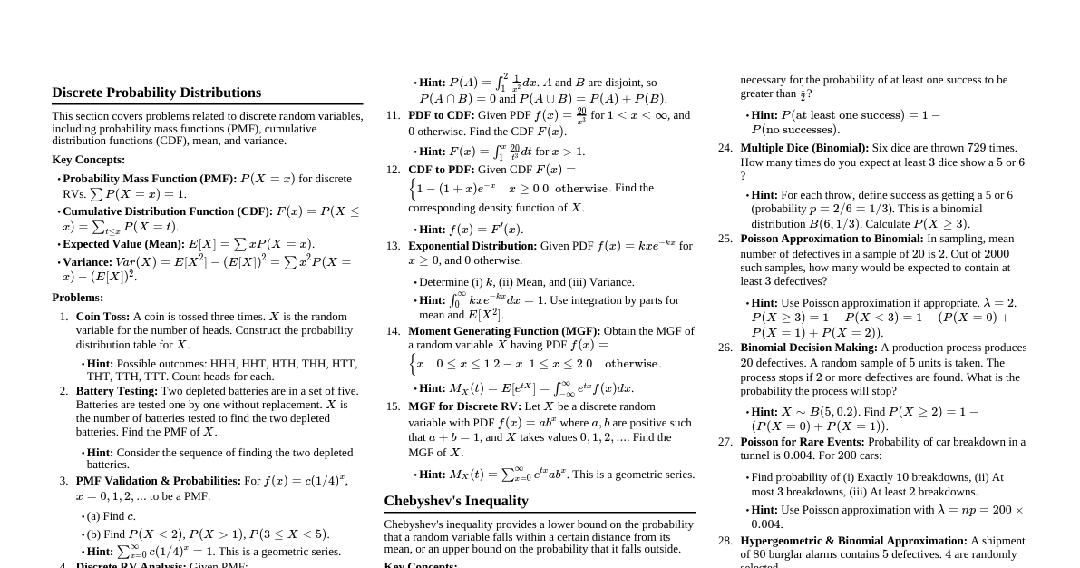
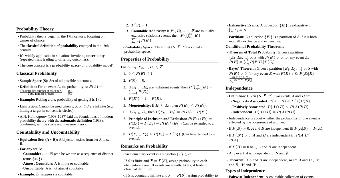
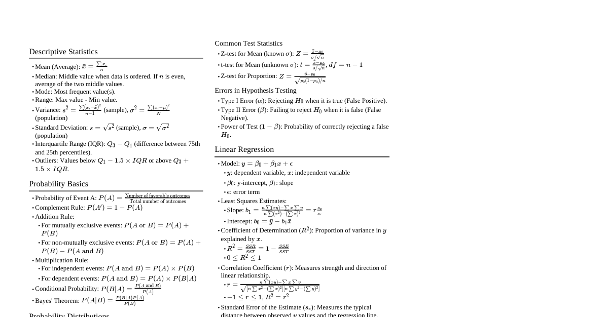
### Probability Basics - **Sample Space ($\Omega$):** The set of all possible outcomes of an experiment. - **Event ($A$):** A subset of the sample space ($\Omega$). - **Probability Measure ($P$):** A function $P: \mathcal{F} \to [0,1]$ (where $\mathcal{F}$ is a $\sigma$-algebra of events) satisfying: 1. $P(A) \ge 0$ for all $A \in \mathcal{F}$ 2. $P(\Omega) = 1$ 3. For any sequence of disjoint events $A_1, A_2, \dots \in \mathcal{F}$, $P(\cup_{i=1}^\infty A_i) = \sum_{i=1}^\infty P(A_i)$. - **Conditional Probability:** $P(A|B) = \frac{P(A \cap B)}{P(B)}$, provided $P(B) > 0$. - **Independence:** Events $A$ and $B$ are independent if $P(A \cap B) = P(A)P(B)$. This implies $P(A|B) = P(A)$ and $P(B|A) = P(B)$. #### Theorem: Bayes' Theorem If $A_1, A_2, \dots, A_n$ are disjoint events such that $\cup_{i=1}^n A_i = \Omega$ and $P(A_i) > 0$ for all $i$, then for any event $B$ with $P(B) > 0$: $$P(A_j|B) = \frac{P(B|A_j)P(A_j)}{\sum_{i=1}^n P(B|A_i)P(A_i)}$$ **Proof:** By the definition of conditional probability, $P(A_j|B) = \frac{P(A_j \cap B)}{P(B)}$. Also, $P(A_j \cap B) = P(B|A_j)P(A_j)$. By the Law of Total Probability, $P(B) = \sum_{i=1}^n P(B \cap A_i) = \sum_{i=1}^n P(B|A_i)P(A_i)$. Substituting these into the first equation yields the theorem. ### Random Variables - **Definition:** A random variable (RV) $X$ is a function $X: \Omega \to \mathbb{R}$ that maps outcomes from the sample space to real numbers. It must be a measurable function. - **Cumulative Distribution Function (CDF):** $F_X(x) = P(X \le x)$ for all $x \in \mathbb{R}$. - Properties: 1. $F_X(x)$ is non-decreasing. 2. $\lim_{x \to -\infty} F_X(x) = 0$ and $\lim_{x \to \infty} F_X(x) = 1$. 3. $F_X(x)$ is right-continuous. - **Probability Mass Function (PMF) for Discrete RVs:** $p_X(x) = P(X=x)$ for all possible values $x$. - $\sum_x p_X(x) = 1$. - $F_X(x) = \sum_{t \le x} p_X(t)$. - **Probability Density Function (PDF) for Continuous RVs:** $f_X(x)$ such that $P(a \le X \le b) = \int_a^b f_X(x) dx$. - Properties: 1. $f_X(x) \ge 0$ for all $x$. 2. $\int_{-\infty}^\infty f_X(x) dx = 1$. - $F_X(x) = \int_{-\infty}^x f_X(t) dt$. If $f_X(x)$ is continuous at $x$, then $F_X'(x) = f_X(x)$. - **Expected Value (Mean):** - Discrete: $E[X] = \sum_x x p_X(x)$ - Continuous: $E[X] = \int_{-\infty}^\infty x f_X(x) dx$ - **Variance:** $Var(X) = E[(X - E[X])^2] = E[X^2] - (E[X])^2$. - **Moment Generating Function (MGF):** $M_X(t) = E[e^{tX}]$. If it exists for $t \in (-h, h)$ for some $h > 0$, then $E[X^k] = M_X^{(k)}(0)$. #### Lemma: Linearity of Expectation For any random variables $X$ and $Y$ and constants $a, b \in \mathbb{R}$: $$E[aX + bY] = aE[X] + bE[Y]$$ **Proof:** For discrete RVs: $E[aX + bY] = \sum_{x,y} (ax+by) P(X=x, Y=y)$ $= \sum_{x,y} ax P(X=x, Y=y) + \sum_{x,y} by P(X=x, Y=y)$ $= a \sum_{x,y} x P(X=x, Y=y) + b \sum_{x,y} y P(X=x, Y=y)$ $= a \sum_x x \sum_y P(X=x, Y=y) + b \sum_y y \sum_x P(X=x, Y=y)$ $= a \sum_x x P(X=x) + b \sum_y y P(Y=y)$ $= aE[X] + bE[Y]$. The proof for continuous RVs involves integrals and is analogous. #### Corollary: Variance of a Sum of Independent RVs If $X$ and $Y$ are independent random variables, then: $$Var(X+Y) = Var(X) + Var(Y)$$ **Proof:** $Var(X+Y) = E[(X+Y)^2] - (E[X+Y])^2$ $= E[X^2 + 2XY + Y^2] - (E[X] + E[Y])^2$ (by linearity of expectation) $= E[X^2] + 2E[XY] + E[Y^2] - (E[X])^2 - 2E[X]E[Y] - (E[Y])^2$ (by linearity of expectation) Since $X$ and $Y$ are independent, $E[XY] = E[X]E[Y]$. So, $Var(X+Y) = E[X^2] + 2E[X]E[Y] + E[Y^2] - (E[X])^2 - 2E[X]E[Y] - (E[Y])^2$ $= (E[X^2] - (E[X])^2) + (E[Y^2] - (E[Y])^2)$ $= Var(X) + Var(Y)$. ### Common Distributions #### Discrete Distributions - **Bernoulli($p$):** $X \sim Ber(p)$, $p_X(x) = p^x (1-p)^{1-x}$ for $x \in \{0,1\}$. $E[X]=p, Var(X)=p(1-p)$. - **Binomial($n, p$):** $X \sim Bin(n, p)$, $p_X(x) = \binom{n}{x} p^x (1-p)^{n-x}$ for $x \in \{0,1,\dots,n\}$. $E[X]=np, Var(X)=np(1-p)$. - **Poisson($\lambda$):** $X \sim Poi(\lambda)$, $p_X(x) = \frac{e^{-\lambda} \lambda^x}{x!}$ for $x \in \{0,1,2,\dots\}$. $E[X]=\lambda, Var(X)=\lambda$. #### Continuous Distributions - **Uniform($a, b$):** $X \sim U(a, b)$, $f_X(x) = \frac{1}{b-a}$ for $x \in [a,b]$. $E[X]=\frac{a+b}{2}, Var(X)=\frac{(b-a)^2}{12}$. - **Normal($\mu, \sigma^2$):** $X \sim N(\mu, \sigma^2)$, $f_X(x) = \frac{1}{\sqrt{2\pi\sigma^2}} e^{-\frac{(x-\mu)^2}{2\sigma^2}}$. $E[X]=\mu, Var(X)=\sigma^2$. - **Exponential($\lambda$):** $X \sim Exp(\lambda)$, $f_X(x) = \lambda e^{-\lambda x}$ for $x > 0$. $E[X]=\frac{1}{\lambda}, Var(X)=\frac{1}{\lambda^2}$. Memoryless property: $P(X > s+t | X > s) = P(X > t)$. #### Theorem: Central Limit Theorem (CLT) Let $X_1, X_2, \dots, X_n$ be a sequence of independent and identically distributed (i.i.d.) random variables with $E[X_i] = \mu$ and $Var(X_i) = \sigma^2 ### Joint Distributions - **Joint CDF:** $F_{X,Y}(x,y) = P(X \le x, Y \le y)$. - **Joint PMF (Discrete):** $p_{X,Y}(x,y) = P(X=x, Y=y)$. - Marginal PMF: $p_X(x) = \sum_y p_{X,Y}(x,y)$. - **Joint PDF (Continuous):** $f_{X,Y}(x,y)$ such that $P((X,Y) \in A) = \iint_A f_{X,Y}(x,y) dx dy$. - Marginal PDF: $f_X(x) = \int_{-\infty}^\infty f_{X,Y}(x,y) dy$. - **Conditional Distributions:** - Discrete: $p_{Y|X}(y|x) = \frac{p_{X,Y}(x,y)}{p_X(x)}$ if $p_X(x) > 0$. - Continuous: $f_{Y|X}(y|x) = \frac{f_{X,Y}(x,y)}{f_X(x)}$ if $f_X(x) > 0$. - **Independence:** $X$ and $Y$ are independent if $F_{X,Y}(x,y) = F_X(x)F_Y(y)$ for all $x,y$. Equivalently, $p_{X,Y}(x,y) = p_X(x)p_Y(y)$ (discrete) or $f_{X,Y}(x,y) = f_X(x)f_Y(y)$ (continuous). - **Covariance:** $Cov(X,Y) = E[(X - E[X])(Y - E[Y])] = E[XY] - E[X]E[Y]$. - **Correlation:** $\rho_{X,Y} = \frac{Cov(X,Y)}{\sqrt{Var(X)Var(Y)}}$. $-1 \le \rho_{X,Y} \le 1$. - **Bivariate Normal Distribution:** If $(X,Y)$ follows a bivariate normal distribution, their joint PDF is: $$f_{X,Y}(x,y) = \frac{1}{2\pi\sigma_X\sigma_Y\sqrt{1-\rho^2}} \exp\left\{-\frac{1}{2(1-\rho^2)}\left[\frac{(x-\mu_X)^2}{\sigma_X^2} - \frac{2\rho(x-\mu_X)(y-\mu_Y)}{\sigma_X\sigma_Y} + \frac{(y-\mu_Y)^2}{\sigma_Y^2}\right]\right\}$$ where $\mu_X, \mu_Y$ are means, $\sigma_X^2, \sigma_Y^2$ are variances, and $\rho$ is the correlation coefficient. If $\rho=0$, $X$ and $Y$ are independent (a unique property of the normal distribution). ### Estimation - **Estimator:** A statistic used to estimate an unknown population parameter. - **Bias:** $Bias(\hat{\theta}) = E[\hat{\theta}] - \theta$. An estimator is unbiased if $Bias(\hat{\theta}) = 0$. - **Mean Squared Error (MSE):** $MSE(\hat{\theta}) = E[(\hat{\theta} - \theta)^2] = Var(\hat{\theta}) + (Bias(\hat{\theta}))^2$. - **Consistency:** An estimator $\hat{\theta}_n$ is consistent if $\hat{\theta}_n \xrightarrow{p} \theta$ (converges in probability) as $n \to \infty$. A sufficient condition for consistency is $\lim_{n \to \infty} MSE(\hat{\theta}_n) = 0$. #### Methods of Estimation ##### 1. Method of Moments (MOM) Equate sample moments to population moments and solve for the parameters. - $m_k = \frac{1}{n}\sum_{i=1}^n X_i^k$ (k-th sample moment) - $\mu_k = E[X^k]$ (k-th population moment) Set $m_k = \mu_k$ for $k=1, \dots, p$ (where $p$ is the number of parameters). ##### 2. Maximum Likelihood Estimation (MLE) Given i.i.d. observations $X_1, \dots, X_n$ from a distribution with PDF/PMF $f(x|\theta)$. The likelihood function is $L(\theta|\mathbf{x}) = \prod_{i=1}^n f(x_i|\theta)$. The MLE $\hat{\theta}_{MLE}$ is the value of $\theta$ that maximizes $L(\theta|\mathbf{x})$ (or equivalently, $\log L(\theta|\mathbf{x})$). #### Theorem: Rao-Blackwell Theorem Let $T$ be a sufficient statistic for $\theta$. Let $\hat{\theta}$ be any unbiased estimator of $\theta$. Then $\hat{\theta}^* = E[\hat{\theta}|T]$ is an unbiased estimator of $\theta$ and $Var(\hat{\theta}^*) \le Var(\hat{\theta})$. If $T$ is also complete, then $\hat{\theta}^*$ is the unique Minimum Variance Unbiased Estimator (MVUE). **Proof (Sketch):** 1. **Unbiasedness:** By the Law of Total Expectation, $E[\hat{\theta}^*] = E[E[\hat{\theta}|T]] = E[\hat{\theta}] = \theta$. So $\hat{\theta}^*$ is unbiased. 2. **Variance:** By the Conditional Variance Formula, $Var(\hat{\theta}) = E[Var(\hat{\theta}|T)] + Var(E[\hat{\theta}|T])$. Since $Var(\hat{\theta}|T) \ge 0$, we have $Var(\hat{\theta}) \ge Var(E[\hat{\theta}|T])$. Thus, $Var(\hat{\theta}) \ge Var(\hat{\theta}^*)$. #### Theorem: Cramer-Rao Lower Bound (CRLB) Under certain regularity conditions, for any unbiased estimator $\hat{\theta}$ of a parameter $\theta$, $$Var(\hat{\theta}) \ge \frac{1}{I(\theta)}$$ where $I(\theta)$ is the Fisher Information: $I(\theta) = E\left[\left(\frac{\partial}{\partial\theta} \log f(X|\theta)\right)^2\right] = -E\left[\frac{\partial^2}{\partial\theta^2} \log f(X|\theta)\right]$. For $n$ i.i.d. observations, $I_n(\theta) = n I(\theta)$. An unbiased estimator that achieves the CRLB is called an efficient estimator. ### Hypothesis Testing - **Null Hypothesis ($H_0$):** A statement about the population parameter that we assume to be true. - **Alternative Hypothesis ($H_1$):** A statement that contradicts $H_0$. - **Test Statistic:** A statistic calculated from sample data used to decide whether to reject $H_0$. - **Type I Error ($\alpha$):** Rejecting $H_0$ when $H_0$ is true ($P(\text{reject } H_0 | H_0 \text{ true})$). Also called significance level. - **Type II Error ($\beta$):** Failing to reject $H_0$ when $H_1$ is true ($P(\text{fail to reject } H_0 | H_1 \text{ true})$). - **Power:** $1 - \beta = P(\text{reject } H_0 | H_1 \text{ true})$. #### Lemma: Neyman-Pearson Lemma To test $H_0: \theta = \theta_0$ against $H_1: \theta = \theta_1$ (simple hypotheses), the most powerful test of size $\alpha$ is given by the likelihood ratio test: Reject $H_0$ if $\frac{L(\theta_1|\mathbf{x})}{L(\theta_0|\mathbf{x})} > k$ for some constant $k$. The constant $k$ is chosen such that $P\left(\frac{L(\theta_1|\mathbf{X})}{L(\theta_0|\mathbf{X})} > k \Big| H_0\right) = \alpha$. **Proof (Sketch):** Let $R$ be the rejection region for the likelihood ratio test, and $R'$ be the rejection region for any other test of the same size $\alpha$. So, $\int_R L(\theta_0|\mathbf{x}) d\mathbf{x} = \int_{R'} L(\theta_0|\mathbf{x}) d\mathbf{x} = \alpha$. We want to show $\int_R L(\theta_1|\mathbf{x}) d\mathbf{x} \ge \int_{R'} L(\theta_1|\mathbf{x}) d\mathbf{x}$. Consider the regions $R \setminus R'$ and $R' \setminus R$. For $\mathbf{x} \in R \setminus R'$, we have $\frac{L(\theta_1|\mathbf{x})}{L(\theta_0|\mathbf{x})} > k$, so $L(\theta_1|\mathbf{x}) > k L(\theta_0|\mathbf{x})$. For $\mathbf{x} \in R' \setminus R$, we have $\frac{L(\theta_1|\mathbf{x})}{L(\theta_0|\mathbf{x})} \le k$, so $L(\theta_1|\mathbf{x}) \le k L(\theta_0|\mathbf{x})$. From the definition of size $\alpha$: $\int_{R \setminus R'} L(\theta_0|\mathbf{x}) d\mathbf{x} = \int_{R' \setminus R} L(\theta_0|\mathbf{x}) d\mathbf{x}$. Multiplying by $k$: $k \int_{R \setminus R'} L(\theta_0|\mathbf{x}) d\mathbf{x} = k \int_{R' \setminus R} L(\theta_0|\mathbf{x}) d\mathbf{x}$. Using the inequalities above, we get: $\int_{R \setminus R'} L(\theta_1|\mathbf{x}) d\mathbf{x} \ge k \int_{R \setminus R'} L(\theta_0|\mathbf{x}) d\mathbf{x}$ $\int_{R' \setminus R} L(\theta_1|\mathbf{x}) d\mathbf{x} \le k \int_{R' \setminus R} L(\theta_0|\mathbf{x}) d\mathbf{x}$ Combining these, we can show that $\int_R L(\theta_1|\mathbf{x}) d\mathbf{x} \ge \int_{R'} L(\theta_1|\mathbf{x}) d\mathbf{x}$, meaning the likelihood ratio test has higher or equal power. ### Confidence Intervals - **Definition:** A $(1-\alpha)100\%$ confidence interval for a parameter $\theta$ is an interval $(L, U)$ such that $P(L \le \theta \le U) = 1-\alpha$. $L$ and $U$ are random variables (statistics). - **For Mean $\mu$ (known $\sigma^2$):** $\bar{X} \pm z_{\alpha/2} \frac{\sigma}{\sqrt{n}}$ - **For Mean $\mu$ (unknown $\sigma^2$):** $\bar{X} \pm t_{n-1, \alpha/2} \frac{S}{\sqrt{n}}$ - **For Proportion $p$ (large $n$):** $\hat{p} \pm z_{\alpha/2} \sqrt{\frac{\hat{p}(1-\hat{p})}{n}}$ #### Theorem: Duality between Confidence Intervals and Hypothesis Tests A $(1-\alpha)100\%$ confidence interval for a parameter $\theta$ corresponds to a two-sided hypothesis test of $H_0: \theta = \theta_0$ vs $H_1: \theta \ne \theta_0$ at significance level $\alpha$. Specifically, $H_0$ is rejected at level $\alpha$ if and only if $\theta_0$ lies outside the $(1-\alpha)100\%$ confidence interval. **Proof (for mean with known variance):** Consider the test $H_0: \mu = \mu_0$ vs $H_1: \mu \ne \mu_0$. The test statistic is $Z = \frac{\bar{X} - \mu_0}{\sigma/\sqrt{n}}$. We reject $H_0$ if $|Z| > z_{\alpha/2}$, which means $\frac{|\bar{X} - \mu_0|}{\sigma/\sqrt{n}} > z_{\alpha/2}$. This inequality can be rewritten as: $\bar{X} - z_{\alpha/2} \frac{\sigma}{\sqrt{n}} > \mu_0$ or $\bar{X} + z_{\alpha/2} \frac{\sigma}{\sqrt{n}} ### Linear Regression - **Simple Linear Regression Model:** $Y_i = \beta_0 + \beta_1 X_i + \epsilon_i$, where $\epsilon_i \sim N(0, \sigma^2)$ are i.i.d. - **Least Squares Estimators:** Minimize $RSS = \sum_{i=1}^n (Y_i - (\beta_0 + \beta_1 X_i))^2$. - $\hat{\beta}_1 = \frac{\sum_{i=1}^n (X_i - \bar{X})(Y_i - \bar{Y})}{\sum_{i=1}^n (X_i - \bar{X})^2} = \frac{S_{XY}}{S_{XX}}$ - $\hat{\beta}_0 = \bar{Y} - \hat{\beta}_1 \bar{X}$ - **Properties of Estimators:** - $E[\hat{\beta}_0] = \beta_0$, $E[\hat{\beta}_1] = \beta_1$ (unbiased) - $Var(\hat{\beta}_1) = \frac{\sigma^2}{\sum (X_i - \bar{X})^2}$ - $Var(\hat{\beta}_0) = \sigma^2 \left(\frac{1}{n} + \frac{\bar{X}^2}{\sum (X_i - \bar{X})^2}\right)$ - **Estimated Variance:** $\hat{\sigma}^2 = S^2 = \frac{RSS}{n-2} = \frac{1}{n-2} \sum_{i=1}^n (Y_i - \hat{Y}_i)^2$. - $E[S^2] = \sigma^2$ (unbiased) - **Coefficient of Determination ($R^2$):** $R^2 = 1 - \frac{RSS}{TSS} = \frac{ESS}{TSS}$, where $TSS = \sum (Y_i - \bar{Y})^2$ (Total Sum of Squares) and $ESS = \sum (\hat{Y}_i - \bar{Y})^2$ (Explained Sum of Squares). $R^2$ measures the proportion of variance in $Y$ explained by $X$. #### Theorem: Gauss-Markov Theorem Under the classical linear model assumptions (linearity, errors have zero mean, constant variance, are uncorrelated), the Ordinary Least Squares (OLS) estimators $\hat{\beta}_0$ and $\hat{\beta}_1$ are the Best Linear Unbiased Estimators (BLUEs). That is, among all linear unbiased estimators, OLS estimators have the smallest variance. **Proof (for $\hat{\beta}_1$):** Let $\hat{\beta}_1 = \sum c_i Y_i$ be any linear unbiased estimator of $\beta_1$. Unbiasedness: $E[\hat{\beta}_1] = E[\sum c_i (\beta_0 + \beta_1 X_i + \epsilon_i)] = \sum c_i \beta_0 + \beta_1 \sum c_i X_i = \beta_1$. For this to hold for any $\beta_0, \beta_1$: $\sum c_i = 0$ $\sum c_i X_i = 1$ Now, $Var(\hat{\beta}_1) = Var(\sum c_i Y_i) = \sum c_i^2 Var(Y_i) = \sigma^2 \sum c_i^2$ (since $Y_i$ are uncorrelated with common variance). We want to minimize $\sum c_i^2$ subject to the constraints. Let $c_i = d_i + k_i$ where $d_i$ are the OLS coefficients for $\hat{\beta}_1$. We know that the OLS coefficients are $d_i = \frac{X_i - \bar{X}}{\sum (X_j - \bar{X})^2}$. We have $\sum d_i = 0$ and $\sum d_i X_i = 1$. $\sum c_i^2 = \sum (d_i + k_i)^2 = \sum d_i^2 + 2 \sum d_i k_i + \sum k_i^2$. From constraints on $c_i$: $\sum k_i = \sum c_i - \sum d_i = 0 - 0 = 0$. $\sum k_i X_i = \sum c_i X_i - \sum d_i X_i = 1 - 1 = 0$. Consider $\sum d_i k_i = \sum \frac{X_i - \bar{X}}{\sum (X_j - \bar{X})^2} k_i = \frac{1}{\sum (X_j - \bar{X})^2} (\sum X_i k_i - \bar{X} \sum k_i)$. Since $\sum k_i = 0$ and $\sum k_i X_i = 0$, we have $\sum d_i k_i = 0$. Therefore, $\sum c_i^2 = \sum d_i^2 + \sum k_i^2$. To minimize $\sum c_i^2$, we must have $\sum k_i^2 = 0$, which implies $k_i = 0$ for all $i$. Thus, the OLS coefficients $d_i$ minimize the variance, making $\hat{\beta}_1$ the BLUE. A similar proof holds for $\hat{\beta}_0$. ### Analysis of Variance (ANOVA) - **Purpose:** To compare means of three or more groups. - **One-Way ANOVA Model:** $Y_{ij} = \mu + \tau_i + \epsilon_{ij}$, where $i=1,\dots,k$ (groups), $j=1,\dots,n_i$ (observations in group $i$). $\epsilon_{ij} \sim N(0, \sigma^2)$ i.i.d. - $H_0: \tau_1 = \tau_2 = \dots = \tau_k = 0$ (all group means are equal) - $H_1:$ At least one $\tau_i \ne 0$ (at least one group mean is different) - **Sums of Squares:** - **Total Sum of Squares (SST):** $\sum_{i=1}^k \sum_{j=1}^{n_i} (Y_{ij} - \bar{Y}_{..})^2$ - **Treatment Sum of Squares (SSTr):** $\sum_{i=1}^k n_i (\bar{Y}_{i.} - \bar{Y}_{..})^2$ (Between-group variation) - **Error Sum of Squares (SSE):** $\sum_{i=1}^k \sum_{j=1}^{n_i} (Y_{ij} - \bar{Y}_{i.})^2$ (Within-group variation) - **Identity:** $SST = SSTr + SSE$ - **Mean Squares:** - **Mean Square for Treatment (MSTr):** $SSTr / (k-1)$ - **Mean Square for Error (MSE):** $SSE / (N-k)$, where $N = \sum n_i$ - **F-statistic:** $F = \frac{MSTr}{MSE}$. Under $H_0$, $F \sim F_{k-1, N-k}$. - **Decision Rule:** Reject $H_0$ if $F > F_{\alpha, k-1, N-k}$. #### Theorem: Expected Mean Squares for One-Way ANOVA Under the one-way ANOVA model with fixed effects $\tau_i$: - $E[MSE] = \sigma^2$ - $E[MSTr] = \sigma^2 + \frac{\sum_{i=1}^k n_i \tau_i^2}{k-1}$ **Proof (for $E[MSE]$):** $SSE = \sum_{i=1}^k \sum_{j=1}^{n_i} (Y_{ij} - \bar{Y}_{i.})^2$. For a fixed group $i$, $\sum_{j=1}^{n_i} (Y_{ij} - \bar{Y}_{i.})^2$ is the sum of squared deviations for that group. We know that for a sample of $n_i$ observations from a normal distribution with variance $\sigma^2$, $\frac{1}{\sigma^2} \sum_{j=1}^{n_i} (Y_{ij} - \bar{Y}_{i.})^2 \sim \chi^2_{n_i-1}$. Therefore, $E\left[\frac{1}{\sigma^2} \sum_{j=1}^{n_i} (Y_{ij} - \bar{Y}_{i.})^2\right] = n_i-1$. So, $E\left[\sum_{j=1}^{n_i} (Y_{ij} - \bar{Y}_{i.})^2\right] = (n_i-1)\sigma^2$. Summing over all groups: $E[SSE] = E\left[\sum_{i=1}^k \sum_{j=1}^{n_i} (Y_{ij} - \bar{Y}_{i.})^2\right] = \sum_{i=1}^k E\left[\sum_{j=1}^{n_i} (Y_{ij} - \bar{Y}_{i.})^2\right] = \sum_{i=1}^k (n_i-1)\sigma^2 = (N-k)\sigma^2$. Finally, $E[MSE] = E\left[\frac{SSE}{N-k}\right] = \frac{1}{N-k} E[SSE] = \frac{1}{N-k} (N-k)\sigma^2 = \sigma^2$. The proof for $E[MSTr]$ is more involved but follows similar principles of expectation and variance for sums of random variables. ### Nonparametric Methods - **Purpose:** Statistical methods that do not rely on strong distributional assumptions (e.g., normality). - **Sign Test:** For testing median differences for paired data. Uses binomial distribution. - **Wilcoxon Signed-Rank Test:** For testing median differences for paired data, considering magnitude and direction of differences. - **Wilcoxon Rank-Sum Test (Mann-Whitney U Test):** For comparing two independent samples' distributions. - **Kruskal-Wallis Test:** Nonparametric alternative to one-way ANOVA for comparing three or more independent samples. - **Spearman's Rank Correlation Coefficient ($r_s$):** Measures the strength and direction of monotonic association between two ranked variables. - $r_s = 1 - \frac{6 \sum d_i^2}{n(n^2-1)}$, where $d_i$ is the difference in ranks for the $i$-th observation. #### Theorem: Asymptotic Distribution of Wilcoxon Rank-Sum Statistic Let $W$ be the Wilcoxon Rank-Sum statistic for comparing two independent samples of sizes $n_1$ and $n_2$. Under the null hypothesis that the two samples come from the same distribution, as $n_1, n_2 \to \infty$: $$Z = \frac{W - E[W]}{\sqrt{Var(W)}} \xrightarrow{d} N(0,1)$$ where $E[W] = \frac{n_1(n_1+n_2+1)}{2}$ and $Var(W) = \frac{n_1 n_2 (n_1+n_2+1)}{12}$. **Proof (Sketch):** The proof relies on the Central Limit Theorem. The Wilcoxon rank-sum statistic $W$ can be expressed as a sum of indicator random variables (or a sum of ranks). When $n_1$ and $n_2$ are large, the distribution of $W$ can be approximated by a normal distribution due to the CLT's applicability to sums of independent (or nearly independent) random variables. The expectation and variance are derived from combinatorial arguments under the null hypothesis that all permutations of ranks are equally likely.