Statistics Final Reviewer

Cheatsheet Content

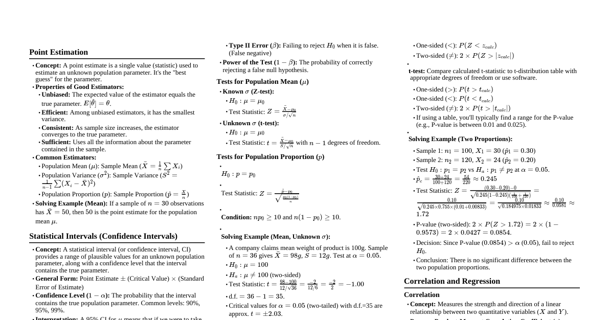
### 1. Point Estimation An estimator is a statistic used to estimate a population parameter. A point estimate is a single numerical value obtained from a sample that serves as the "best guess" or an approximation of the true population parameter. #### Properties of Good Estimators: - **Unbiased:** An estimator is unbiased if its expected value is equal to the true population parameter. $E[\hat{\theta}] = \theta$. - **Efficient:** Among unbiased estimators, the one with the smallest variance is considered most efficient. This means its estimates are clustered more closely around the true parameter. - **Consistent:** As the sample size $n$ increases, the estimator converges in probability to the true parameter. This means the probability that the estimator is far from the true parameter becomes very small as $n \to \infty$. - **Sufficient:** An estimator is sufficient if it uses all the information about the parameter that is contained in the sample. #### Common Point Estimators: - **Population Mean ($\mu$):** Sample Mean ($\bar{x}$) - Formula: $\bar{x} = \frac{\sum x_i}{n}$ - **Population Proportion ($p$):** Sample Proportion ($\hat{p}$) - Formula: $\hat{p} = \frac{x}{n}$ (where $x$ is the number of successes) - **Population Variance ($\sigma^2$):** Sample Variance ($s^2$) - Formula: $s^2 = \frac{\sum (x_i - \bar{x})^2}{n-1}$ (using $n-1$ for unbiased estimation) - **Population Standard Deviation ($\sigma$):** Sample Standard Deviation ($s$) - Formula: $s = \sqrt{\frac{\sum (x_i - \bar{x})^2}{n-1}}$ #### Example (Solving): Suppose we take a random sample of 10 students' test scores: 85, 90, 78, 92, 88, 75, 81, 95, 83, 89. - **Point estimate for the population mean score ($\mu$):** $\bar{x} = \frac{85+90+78+92+88+75+81+95+83+89}{10} = \frac{856}{10} = 85.6$ So, 85.6 is our point estimate for the average test score of all students. - **Point estimate for the population standard deviation ($\sigma$):** First, calculate $s^2$: $\sum (x_i - \bar{x})^2 = (85-85.6)^2 + (90-85.6)^2 + ... + (89-85.6)^2 = 369.6$ $s^2 = \frac{369.6}{10-1} = \frac{369.6}{9} = 41.067$ $s = \sqrt{41.067} \approx 6.408$ So, 6.408 is our point estimate for the standard deviation of test scores. ### 2. Statistical Intervals (Confidence Intervals) A statistical interval, specifically a confidence interval (CI), provides a range of values within which the true population parameter is likely to lie, with a certain level of confidence. It addresses the limitation of point estimates (being a single value) by quantifying the uncertainty. #### General Form of a Confidence Interval: Point Estimate $\pm$ (Critical Value $\times$ Standard Error of the Estimator) #### Key Components: - **Point Estimate:** The sample statistic used to estimate the parameter. - **Confidence Level (CL):** The probability that the interval contains the true population parameter. Common levels are 90%, 95%, 99%. - **Alpha ($\alpha$):** The significance level, $\alpha = 1 - CL$. Represents the probability that the interval *does not* contain the true parameter. - **Critical Value:** A value from a standard distribution (e.g., Z-distribution, t-distribution) that corresponds to the chosen confidence level. It defines the number of standard errors away from the mean that captures the middle $CL\%$ of the distribution. - For large samples or known population standard deviation ($\sigma$): Z-score ($z_{\alpha/2}$) - For small samples and unknown population standard deviation ($\sigma$): t-score ($t_{\alpha/2, df}$) - **Standard Error (SE):** The standard deviation of the sampling distribution of the point estimator. It measures the precision of the estimate. #### Confidence Interval for Population Mean ($\mu$): - **Known $\sigma$ (or large $n \ge 30$):** $\bar{x} \pm z_{\alpha/2} \frac{\sigma}{\sqrt{n}}$ - **Unknown $\sigma$ (and small $n ### 3. Test of Hypothesis in Single Sample Hypothesis testing is a formal procedure for evaluating competing claims about a population parameter using sample data. It helps determine if there is enough evidence to reject a null hypothesis in favor of an alternative hypothesis. #### Key Concepts: 1. **Null Hypothesis ($H_0$):** A statement of no effect, no difference, or no change. It's the default assumption. It always contains an equality ($=$, $\le$, $\ge$). * Example: $H_0: \mu = 50$ (The population mean is 50). 2. **Alternative Hypothesis ($H_1$ or $H_a$):** A statement that contradicts the null hypothesis. It's what we are trying to find evidence for. It never contains an equality ($ $, $\ne$). * Example: $H_1: \mu \ne 50$ (Two-tailed test) * Example: $H_1: \mu > 50$ (Right-tailed test) * Example: $H_1: \mu ### 4. Statistical Inference in Two Samples This involves comparing two population parameters (means, proportions, variances) based on independent or dependent samples. #### Comparing Two Population Means ($\mu_1 - \mu_2$): **A. Independent Samples:** Data from one sample does not influence the other. 1. **Known Population Variances ($\sigma_1^2, \sigma_2^2$):** * **Hypotheses:** * $H_0: \mu_1 - \mu_2 = D_0$ (often $D_0=0$, meaning $\mu_1 = \mu_2$) * $H_1: \mu_1 - \mu_2 \ne D_0$ or $>$ or $ $ or $ $ or $ $):** P-value = $P(Z > z_{calc})$ * **Left-tailed ($H_1: |z_{calc}|)$ * Use a standard normal (Z) table or calculator. * **For t-tests:** * **Right-tailed ($H_1: >$):** P-value = $P(T > t_{calc})$ * **Left-tailed ($H_1: |t_{calc}|)$ * Use a t-distribution table with the correct degrees of freedom ($df$) or a calculator. Since t-tables usually provide critical values for specific $\alpha$ and $df$, finding an exact P-value requires software or interpolation. However, you can state whether the P-value is less than or greater than a given $\alpha$ by comparing $t_{calc}$ to $t_{\alpha, df}$. #### Example (Solving - Two Proportions): A survey is conducted to compare the proportion of people who prefer brand A in City 1 vs. City 2. - City 1: $n_1 = 200$, $x_1 = 120$ prefer Brand A ($\hat{p}_1 = 120/200 = 0.60$) - City 2: $n_2 = 150$, $x_2 = 75$ prefer Brand A ($\hat{p}_2 = 75/150 = 0.50$) Test if there's a significant difference in preference at $\alpha = 0.05$. 1. **Hypotheses:** * $H_0: p_1 - p_2 = 0$ (No difference in preference) * $H_1: p_1 - p_2 \ne 0$ (There is a difference - Two-tailed) 2. **Significance Level:** $\alpha = 0.05$. 3. **Test Statistic:** Z-test for two proportions. First, calculate pooled proportion: $\hat{p} = \frac{120 + 75}{200 + 150} = \frac{195}{350} \approx 0.557$ 4. **Calculate Test Statistic:** $Z = \frac{(0.60 - 0.50) - 0}{\sqrt{0.557(1-0.557)(\frac{1}{200} + \frac{1}{150})}}$ $Z = \frac{0.10}{\sqrt{0.557 \times 0.443 \times (0.005 + 0.006667)}}$ $Z = \frac{0.10}{\sqrt{0.2467 \times 0.011667}} = \frac{0.10}{\sqrt{0.002878}} = \frac{0.10}{0.0536} \approx 1.866$ 5. **Find P-value:** This is a two-tailed test. P-value = $2 \times P(Z > |1.866|) = 2 \times P(Z > 1.866)$. From Z-table, $P(Z > 1.866) \approx 1 - 0.9689 = 0.0311$. P-value = $2 \times 0.0311 = 0.0622$. 6. **Make a Decision:** Since P-value $(0.0622) > \alpha (0.05)$, we fail to reject $H_0$. 7. **Conclusion:** There is not enough evidence at the 0.05 significance level to conclude that there is a significant difference in brand preference between City 1 and City 2. ### 5. Correlation and Regression #### Correlation Correlation quantifies the strength and direction of a linear relationship between two quantitative variables. - **Pearson Product-Moment Correlation Coefficient ($r$):** - Measures the linear association between two variables $X$ and $Y$. - Formula: $r = \frac{\sum (x_i - \bar{x})(y_i - \bar{y})}{\sqrt{\sum (x_i - \bar{x})^2 \sum (y_i - \bar{y})^2}} = \frac{S_{xy}}{S_x S_y}$ - Range: $-1 \le r \le 1$. - $r = 1$: Perfect positive linear correlation. - $r = -1$: Perfect negative linear correlation. - $r = 0$: No linear correlation. - **Coefficient of Determination ($r^2$):** Represents the proportion of the variance in the dependent variable ($Y$) that is predictable from the independent variable ($X$). $0 \le r^2 \le 1$. #### Regression (Simple Linear Regression) Regression analysis models the relationship between a dependent variable ($Y$) and one or more independent variables ($X$). Simple linear regression uses one independent variable to predict the dependent variable. - **Model:** $Y = \beta_0 + \beta_1 X + \epsilon$ - $Y$: Dependent variable - $X$: Independent variable - $\beta_0$: Y-intercept (value of Y when X=0) - $\beta_1$: Slope (change in Y for a one-unit change in X) - $\epsilon$: Error term (random variation not explained by the model) - **Estimated Regression Line (Least Squares Regression Line):** $\hat{y} = b_0 + b_1 x$ - $\hat{y}$: Predicted value of Y for a given X. - $b_1$: Sample estimate of the slope $\beta_1$. - $b_0$: Sample estimate of the Y-intercept $\beta_0$. - **Formulas for $b_1$ and $b_0$ (Least Squares Estimates):** - $b_1 = \frac{\sum (x_i - \bar{x})(y_i - \bar{y})}{\sum (x_i - \bar{x})^2} = r \frac{S_y}{S_x}$ - $b_0 = \bar{y} - b_1 \bar{x}$ - **Assumptions of Linear Regression:** 1. **Linearity:** The relationship between X and Y is linear. 2. **Independence of Errors:** Residuals ($\epsilon$) are independent. 3. **Normality of Errors:** Residuals are normally distributed. 4. **Homoscedasticity:** Constant variance of errors across all levels of X. - **Interpretation of $b_1$:** For every one-unit increase in $X$, the predicted value of $Y$ changes by $b_1$ units. - **Interpretation of $b_0$:** The predicted value of $Y$ when $X=0$. (Only meaningful if $X=0$ is within the range of observed X values). #### Example (Solving): Consider the relationship between advertising expenditure (X, in thousands of dollars) and sales revenue (Y, in thousands of dollars) for 5 months. | Month | X (Ads) | Y (Sales) | |-------|---------|-----------| | 1 | 1 | 10 | | 2 | 2 | 12 | | 3 | 3 | 15 | | 4 | 4 | 16 | | 5 | 5 | 18 | Calculations: - $\sum x_i = 15$, $\bar{x} = 3$ - $\sum y_i = 71$, $\bar{y} = 14.2$ - $\sum (x_i - \bar{x})^2 = (1-3)^2 + (2-3)^2 + (3-3)^2 + (4-3)^2 + (5-3)^2 = 4+1+0+1+4 = 10$ - $\sum (y_i - \bar{y})^2 = (10-14.2)^2 + ... + (18-14.2)^2 = 45.2$ - $\sum (x_i - \bar{x})(y_i - \bar{y}) = (-2)(-4.2) + (-1)(-2.2) + (0)(0.8) + (1)(1.8) + (2)(3.8) = 8.4 + 2.2 + 0 + 1.8 + 7.6 = 20$ 1. **Calculate Correlation Coefficient ($r$):** $r = \frac{20}{\sqrt{10 \times 45.2}} = \frac{20}{\sqrt{452}} = \frac{20}{21.26} \approx 0.9416$ Interpretation: There is a strong positive linear relationship between advertising expenditure and sales revenue. 2. **Calculate Regression Line ($\hat{y} = b_0 + b_1 x$):** - **Slope ($b_1$):** $b_1 = \frac{\sum (x_i - \bar{x})(y_i - \bar{y})}{\sum (x_i - \bar{x})^2} = \frac{20}{10} = 2$ - **Y-intercept ($b_0$):** $b_0 = \bar{y} - b_1 \bar{x} = 14.2 - 2 \times 3 = 14.2 - 6 = 8.2$ - **Regression Equation:** $\hat{y} = 8.2 + 2x$ 3. **Interpretation:** - **Slope ($b_1 = 2$):** For every additional thousand dollars spent on advertising, sales revenue is predicted to increase by 2 thousand dollars. - **Y-intercept ($b_0 = 8.2$):** When no money is spent on advertising (X=0), the predicted sales revenue is 8.2 thousand dollars. 4. **Prediction:** If the company spends $3.5 thousand on advertising, what are the predicted sales? $\hat{y} = 8.2 + 2(3.5) = 8.2 + 7 = 15.2$ Predicted sales revenue is 15.2 thousand dollars. ### 6. Joint Probability Distribution A joint probability distribution describes the probabilities of two or more random variables occurring simultaneously. #### A. Joint Probability Mass Function (PMF) for Discrete Variables: - For two discrete random variables $X$ and $Y$, the joint PMF is $P(X=x, Y=y) = p(x,y)$. - Properties: 1. $0 \le p(x,y) \le 1$ for all $(x,y)$. 2. $\sum_{x} \sum_{y} p(x,y) = 1$. - **Marginal Probability Mass Function:** - For $X$: $p_X(x) = \sum_{y} p(x,y)$ - For $Y$: $p_Y(y) = \sum_{x} p(x,y)$ - **Conditional Probability Mass Function:** - $P(Y=y | X=x) = \frac{p(x,y)}{p_X(x)}$, provided $p_X(x) > 0$. - $P(X=x | Y=y) = \frac{p(x,y)}{p_Y(y)}$, provided $p_Y(y) > 0$. - **Independence:** Two discrete random variables $X$ and $Y$ are independent if and only if $p(x,y) = p_X(x) p_Y(y)$ for all possible $(x,y)$ values. #### B. Joint Probability Density Function (PDF) for Continuous Variables: - For two continuous random variables $X$ and $Y$, the joint PDF is $f(x,y)$. - Properties: 1. $f(x,y) \ge 0$ for all $(x,y)$. 2. $\int_{-\infty}^{\infty} \int_{-\infty}^{\infty} f(x,y) \,dx\,dy = 1$. - **Marginal Probability Density Function:** - For $X$: $f_X(x) = \int_{-\infty}^{\infty} f(x,y) \,dy$ - For $Y$: $f_Y(y) = \int_{-\infty}^{\infty} f(x,y) \,dx$ - **Conditional Probability Density Function:** - $f_{Y|X}(y|x) = \frac{f(x,y)}{f_X(x)}$, provided $f_X(x) > 0$. - $f_{X|Y}(x|y) = \frac{f(x,y)}{f_Y(y)}$, provided $f_Y(y) > 0$. - **Independence:** Two continuous random variables $X$ and $Y$ are independent if and only if $f(x,y) = f_X(x) f_Y(y)$ for all possible $(x,y)$ values. #### Expected Values and Covariance: - **Expected Value of a Function of X and Y:** - Discrete: $E[g(X,Y)] = \sum_{x} \sum_{y} g(x,y) p(x,y)$ - Continuous: $E[g(X,Y)] = \int_{-\infty}^{\infty} \int_{-\infty}^{\infty} g(x,y) f(x,y) \,dx\,dy$ - **Covariance:** Measures the degree to which two variables change together. $Cov(X,Y) = E[(X - E[X])(Y - E[Y])] = E[XY] - E[X]E[Y]$ - Positive covariance: X and Y tend to move in the same direction. - Negative covariance: X and Y tend to move in opposite directions. - Zero covariance: No linear relationship (does not imply independence). - **Correlation Coefficient ($\rho$):** Standardized measure of linear association (population equivalent of $r$). $\rho = \frac{Cov(X,Y)}{\sigma_X \sigma_Y}$ - Range: $-1 \le \rho \le 1$. #### Example (Discrete Joint PMF): A company has two projects, A and B. Let X be the number of successful outcomes for Project A (0 or 1) and Y be the number of successful outcomes for Project B (0 or 1). The joint PMF is given by: | $P(X=x, Y=y)$ | Y=0 | Y=1 | $p_X(x)$ | |---------------|-------|-------|----------| | **X=0** | 0.1 | 0.2 | 0.3 | | **X=1** | 0.3 | 0.4 | 0.7 | | **$p_Y(y)$** | 0.4 | 0.6 | 1.0 | 1. **Verify properties:** All $p(x,y) \ge 0$. Sum of all $p(x,y) = 0.1+0.2+0.3+0.4 = 1.0$. (Properties satisfied). 2. **Calculate Marginal PMFs:** - $p_X(0) = P(X=0, Y=0) + P(X=0, Y=1) = 0.1 + 0.2 = 0.3$ - $p_X(1) = P(X=1, Y=0) + P(X=1, Y=1) = 0.3 + 0.4 = 0.7$ - $p_Y(0) = P(X=0, Y=0) + P(X=1, Y=0) = 0.1 + 0.3 = 0.4$ - $p_Y(1) = P(X=0, Y=1) + P(X=1, Y=1) = 0.2 + 0.4 = 0.6$ (These are already in the table margins). 3. **Calculate Conditional Probabilities:** - $P(Y=1 | X=0) = \frac{P(X=0, Y=1)}{P(X=0)} = \frac{0.2}{0.3} = \frac{2}{3} \approx 0.667$ (If Project A fails, the probability Project B succeeds is 2/3). - $P(X=1 | Y=1) = \frac{P(X=1, Y=1)}{P(Y=1)} = \frac{0.4}{0.6} = \frac{2}{3} \approx 0.667$ (If Project B succeeds, the probability Project A succeeds is 2/3). 4. **Check for Independence:** - Is $P(X=0, Y=0) = P(X=0) \times P(Y=0)$? $0.1 \ne 0.3 \times 0.4 = 0.12$. - Since $p(0,0) \ne p_X(0)p_Y(0)$, X and Y are NOT independent. 5. **Calculate Expected Values and Covariance:** - $E[X] = (0 \times 0.3) + (1 \times 0.7) = 0.7$ - $E[Y] = (0 \times 0.4) + (1 \times 0.6) = 0.6$ - $E[XY] = (0 \times 0 \times 0.1) + (0 \times 1 \times 0.2) + (1 \times 0 \times 0.3) + (1 \times 1 \times 0.4) = 0.4$ - $Cov(X,Y) = E[XY] - E[X]E[Y] = 0.4 - (0.7 \times 0.6) = 0.4 - 0.42 = -0.02$ - The negative covariance indicates a slight tendency for them to move in opposite directions, although the value is small.