Statistics Final Review

Cheatsheet Content

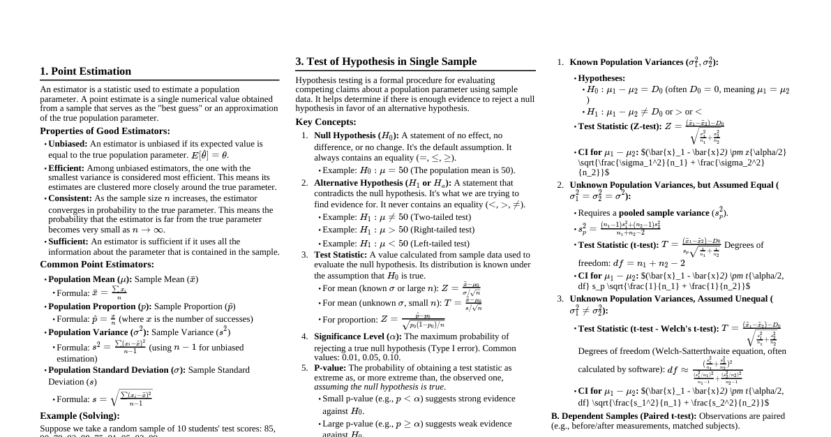
### Point Estimation - **Concept:** A point estimate is a single value (statistic) used to estimate an unknown population parameter. It's the "best guess" for the parameter. - **Properties of Good Estimators:** - **Unbiased:** The expected value of the estimator equals the true parameter. $E[\hat{\theta}] = \theta$. - **Efficient:** Among unbiased estimators, it has the smallest variance. - **Consistent:** As sample size increases, the estimator converges to the true parameter. - **Sufficient:** Uses all the information about the parameter contained in the sample. - **Common Estimators:** - Population Mean ($\mu$): Sample Mean ($\bar{X} = \frac{1}{n}\sum X_i$) - Population Variance ($\sigma^2$): Sample Variance ($S^2 = \frac{1}{n-1}\sum (X_i - \bar{X})^2$) - Population Proportion ($p$): Sample Proportion ($\hat{p} = \frac{X}{n}$) - **Solving Example (Mean):** If a sample of $n=30$ observations has $\bar{X}=50$, then $50$ is the point estimate for the population mean $\mu$. ### Statistical Intervals (Confidence Intervals) - **Concept:** A statistical interval (or confidence interval, CI) provides a range of plausible values for an unknown population parameter, along with a confidence level that the interval contains the true parameter. - **General Form:** Point Estimate $\pm$ (Critical Value) $\times$ (Standard Error of Estimate) - **Confidence Level ($1-\alpha$):** The probability that the interval contains the true population parameter. Common levels: 90%, 95%, 99%. - **Interpretation:** A 95% CI for $\mu$ means that if we were to take many samples and construct a CI for each, about 95% of these intervals would contain the true $\mu$. It does NOT mean there is a 95% chance the true $\mu$ is in THIS interval. - **Types of Confidence Intervals:** #### CI for Population Mean ($\mu$) - **Known $\sigma$:** - Formula: $\bar{X} \pm Z_{\alpha/2} \frac{\sigma}{\sqrt{n}}$ - $Z_{\alpha/2}$ is the critical value from the standard normal distribution. - **Unknown $\sigma$ (use $S$):** - Formula: $\bar{X} \pm t_{\alpha/2, n-1} \frac{S}{\sqrt{n}}$ - $t_{\alpha/2, n-1}$ is the critical value from the t-distribution with $n-1$ degrees of freedom. #### CI for Population Proportion ($p$) - **Formula:** $\hat{p} \pm Z_{\alpha/2} \sqrt{\frac{\hat{p}(1-\hat{p})}{n}}$ - **Condition:** $n\hat{p} \ge 10$ and $n(1-\hat{p}) \ge 10$ for normal approximation. - **Solving Example (Mean, Unknown $\sigma$):** - Sample: $n=25$, $\bar{X}=60$, $S=10$. Confidence Level: 95%. - $\alpha = 0.05$, $\alpha/2 = 0.025$. d.f. $= n-1 = 24$. - From t-table, $t_{0.025, 24} = 2.064$. - CI: $60 \pm 2.064 \frac{10}{\sqrt{25}} = 60 \pm 2.064 \times 2 = 60 \pm 4.128$ - Interval: $(55.872, 64.128)$ ### Hypothesis Testing in Single Sample - **Concept:** A formal procedure to decide whether to reject a claim (null hypothesis) about a population parameter based on sample data. - **Key Components:** 1. **Null Hypothesis ($H_0$):** A statement of no effect, no difference, or no change. Always contains an equality ($=, \le, \ge$). 2. **Alternative Hypothesis ($H_a$ or $H_1$):** A statement that contradicts $H_0$. Can be one-sided ($ $) or two-sided ($\ne$). 3. **Test Statistic:** A value calculated from sample data used to evaluate the null hypothesis. It follows a known distribution (Z, t, $\chi^2$, F). 4. **Significance Level ($\alpha$):** The maximum probability of rejecting a true null hypothesis (Type I error). Common values: 0.01, 0.05, 0.10. 5. **P-value:** The probability of observing a test statistic as extreme as, or more extreme than, the one calculated from the sample, assuming $H_0$ is true. 6. **Decision Rule:** - **P-value approach:** If P-value $\le \alpha$, reject $H_0$. - **Critical Value approach:** If test statistic falls in the rejection region, reject $H_0$. 7. **Conclusion:** State the decision in the context of the problem. - **Types of Errors:** - **Type I Error ($\alpha$):** Rejecting $H_0$ when it is true. (False positive) - **Type II Error ($\beta$):** Failing to reject $H_0$ when it is false. (False negative) - **Power of the Test ($1-\beta$):** The probability of correctly rejecting a false null hypothesis. #### Tests for Population Mean ($\mu$) - **Known $\sigma$ (Z-test):** - $H_0: \mu = \mu_0$ - Test Statistic: $Z = \frac{\bar{X} - \mu_0}{\sigma/\sqrt{n}}$ - **Unknown $\sigma$ (t-test):** - $H_0: \mu = \mu_0$ - Test Statistic: $t = \frac{\bar{X} - \mu_0}{S/\sqrt{n}}$ with $n-1$ degrees of freedom. #### Tests for Population Proportion ($p$) - **$H_0: p = p_0$** - Test Statistic: $Z = \frac{\hat{p} - p_0}{\sqrt{\frac{p_0(1-p_0)}{n}}}$ - **Condition:** $np_0 \ge 10$ and $n(1-p_0) \ge 10$. - **Solving Example (Mean, Unknown $\sigma$):** - A company claims mean weight of product is 100g. Sample of $n=36$ gives $\bar{X}=98g$, $S=12g$. Test at $\alpha=0.05$. - $H_0: \mu = 100$ - $H_a: \mu \ne 100$ (two-sided) - Test Statistic: $t = \frac{98 - 100}{12/\sqrt{36}} = \frac{-2}{12/6} = \frac{-2}{2} = -1.00$ - d.f. $= 36-1 = 35$. - Critical values for $\alpha=0.05$ (two-tailed) with d.f.=35 are approx. $t = \pm 2.03$. - P-value: $P(t 1.00)$ with d.f.=35. Using t-table/software, P-value is approx. $0.325$. - Decision: Since P-value ($0.325$) $> \alpha$ ($0.05$), we fail to reject $H_0$. - Conclusion: There is not enough evidence to conclude that the mean weight is different from 100g. ### Statistical Inference in Two Samples - **Concept:** Comparing two population parameters (means or proportions) based on two independent samples. #### Inference for Two Population Means ($\mu_1 - \mu_2$) ##### 1. Independent Samples, $\sigma_1, \sigma_2$ Known (Z-test) - **Hypotheses:** - $H_0: \mu_1 = \mu_2$ (or $\mu_1 - \mu_2 = D_0$, typically $D_0=0$) - $H_a: \mu_1 \ne \mu_2$ or $\mu_1 > \mu_2$ or $\mu_1 p_2$ or $p_1 $): $P(Z > z_{calc})$ - One-sided ($ |z_{calc}|)$ - **t-test:** Compare calculated t-statistic to t-distribution table with appropriate degrees of freedom or use software. - One-sided ($>$): $P(t > t_{calc})$ - One-sided ($ |t_{calc}|)$ - If using a table, you'll typically find a range for the P-value (e.g., P-value is between 0.01 and 0.025). - **Solving Example (Two Proportions):** - Sample 1: $n_1=100$, $X_1=30$ ($\hat{p}_1 = 0.30$) - Sample 2: $n_2=120$, $X_2=24$ ($\hat{p}_2 = 0.20$) - Test $H_0: p_1 = p_2$ vs $H_a: p_1 \ne p_2$ at $\alpha=0.05$. - $\hat{p}_c = \frac{30+24}{100+120} = \frac{54}{220} \approx 0.245$ - Test Statistic: $Z = \frac{(0.30 - 0.20) - 0}{\sqrt{0.245(1-0.245)(\frac{1}{100} + \frac{1}{120})}} = \frac{0.10}{\sqrt{0.245 \times 0.755 \times (0.01 + 0.00833)}} = \frac{0.10}{\sqrt{0.184975 \times 0.01833}} \approx \frac{0.10}{0.0581} \approx 1.72$ - P-value (two-sided): $2 \times P(Z > 1.72) = 2 \times (1 - 0.9573) = 2 \times 0.0427 = 0.0854$. - Decision: Since P-value ($0.0854$) $> \alpha$ ($0.05$), fail to reject $H_0$. - Conclusion: There is no significant difference between the two population proportions. ### Correlation and Regression #### Correlation - **Concept:** Measures the strength and direction of a linear relationship between two quantitative variables ($X$ and $Y$). - **Pearson Product-Moment Correlation Coefficient ($r$):** - Formula: $r = \frac{\sum (x_i - \bar{x})(y_i - \bar{y})}{\sqrt{\sum (x_i - \bar{x})^2 \sum (y_i - \bar{y})^2}} = \frac{S_{xy}}{S_x S_y}$ - Range: $-1 \le r \le 1$ - Interpretation: - $r=1$: Perfect positive linear relationship - $r=-1$: Perfect negative linear relationship - $r=0$: No linear relationship (may have non-linear) - Closer to $\pm 1$, stronger the relationship. - **Coefficient of Determination ($r^2$):** - Concept: The proportion of the total variation in the dependent variable ($Y$) that is explained by the linear relationship with the independent variable ($X$). - Range: $0 \le r^2 \le 1$. - Example: If $r^2 = 0.64$, then 64% of the variation in $Y$ can be explained by $X$. - **Causation:** Correlation does NOT imply causation. #### Simple Linear Regression - **Concept:** Models the linear relationship between a dependent variable ($Y$) and a single independent variable ($X$). Used for prediction and understanding the relationship. - **Regression Equation (Least Squares Line):** $\hat{Y} = b_0 + b_1 X$ - $\hat{Y}$: Predicted value of the dependent variable - $b_0$: Y-intercept (value of $\hat{Y}$ when $X=0$) - $b_1$: Slope (change in $\hat{Y}$ for a one-unit increase in $X$) - **Formulas for Coefficients:** - Slope: $b_1 = \frac{\sum (x_i - \bar{x})(y_i - \bar{y})}{\sum (x_i - \bar{x})^2} = \frac{S_{xy}}{S_{xx}}$ - Intercept: $b_0 = \bar{Y} - b_1 \bar{X}$ - **Assumptions of Linear Regression (for inference):** 1. **Linearity:** The relationship between $X$ and $Y$ is linear. 2. **Independence:** Residuals are independent. 3. **Normality:** Residuals are normally distributed. 4. **Equal Variance (Homoscedasticity):** Variance of residuals is constant across all levels of $X$. - **Residuals:** $e_i = Y_i - \hat{Y}_i$. The difference between observed and predicted values. - **Standard Error of the Estimate ($S_e$):** Measures the typical distance between observed $Y$ values and the regression line. $S_e = \sqrt{\frac{\sum (Y_i - \hat{Y}_i)^2}{n-2}}$ #### Solving Example (Regression): - Given data points $(x,y)$: $(1,2), (2,4), (3,5)$ - $\bar{X} = 2$, $\bar{Y} = 11/3 \approx 3.67$ - $\sum (x_i - \bar{x})^2 = (1-2)^2 + (2-2)^2 + (3-2)^2 = 1+0+1 = 2$ - $\sum (y_i - \bar{y})^2 = (2-11/3)^2 + (4-11/3)^2 + (5-11/3)^2 = (-5/3)^2 + (1/3)^2 + (4/3)^2 = 25/9 + 1/9 + 16/9 = 42/9 \approx 4.67$ - $\sum (x_i - \bar{x})(y_i - \bar{y}) = (1-2)(2-11/3) + (2-2)(4-11/3) + (3-2)(5-11/3) = (-1)(-5/3) + (0)(1/3) + (1)(4/3) = 5/3 + 0 + 4/3 = 9/3 = 3$ - **Slope ($b_1$):** $b_1 = \frac{3}{2} = 1.5$ - **Intercept ($b_0$):** $b_0 = 11/3 - 1.5(2) = 11/3 - 3 = 11/3 - 9/3 = 2/3 \approx 0.67$ - **Regression Equation:** $\hat{Y} = 0.67 + 1.5X$ - **Correlation ($r$):** $r = \frac{3}{\sqrt{2 \times 42/9}} = \frac{3}{\sqrt{84/9}} = \frac{3}{\sqrt{9.33}} \approx \frac{3}{3.055} \approx 0.982$ (strong positive linear relationship) ### Joint Probability Distribution - **Concept:** Describes the probability of two or more random variables occurring simultaneously. - **Joint Probability Mass Function (PMF)** for discrete random variables: $P(X=x, Y=y) = p(x,y)$ - **Joint Probability Density Function (PDF)** for continuous random variables: $f(x,y)$ - **Key Properties:** - For discrete: $\sum_x \sum_y p(x,y) = 1$ - For continuous: $\int_{-\infty}^{\infty} \int_{-\infty}^{\infty} f(x,y) \, dx \, dy = 1$ - $p(x,y) \ge 0$ or $f(x,y) \ge 0$ for all $x,y$. #### Marginal Probability Distributions - **Concept:** The probability distribution of a single random variable in a joint distribution. - **For Discrete Variables:** - $P(X=x) = p_X(x) = \sum_y p(x,y)$ (summing across rows for X) - $P(Y=y) = p_Y(y) = \sum_x p(x,y)$ (summing down columns for Y) - **For Continuous Variables:** - $f_X(x) = \int_{-\infty}^{\infty} f(x,y) \, dy$ - $f_Y(y) = \int_{-\infty}^{\infty} f(x,y) \, dx$ #### Conditional Probability Distributions - **Concept:** The probability distribution of one variable given that another variable has taken a specific value. - **For Discrete Variables:** - $P(Y=y | X=x) = \frac{p(x,y)}{p_X(x)}$, provided $p_X(x) > 0$ - $P(X=x | Y=y) = \frac{p(x,y)}{p_Y(y)}$, provided $p_Y(y) > 0$ - **For Continuous Variables:** - $f_{Y|X}(y|x) = \frac{f(x,y)}{f_X(x)}$, provided $f_X(x) > 0$ - $f_{X|Y}(x|y) = \frac{f(x,y)}{f_Y(y)}$, provided $f_Y(y) > 0$ #### Independence of Random Variables - **Concept:** Two random variables $X$ and $Y$ are independent if their joint distribution is the product of their marginal distributions. - **For Discrete Variables:** $p(x,y) = p_X(x) \cdot p_Y(y)$ for all $x,y$. - **For Continuous Variables:** $f(x,y) = f_X(x) \cdot f_Y(y)$ for all $x,y$. - If $X$ and $Y$ are independent, then $P(Y=y | X=x) = P(Y=y)$ and $f_{Y|X}(y|x) = f_Y(y)$. #### Covariance and Correlation - **Covariance (Cov($X,Y$)):** Measures the direction of the linear relationship between two variables. - $\text{Cov}(X,Y) = E[(X - E[X])(Y - E[Y])] = E[XY] - E[X]E[Y]$ - Positive covariance: $X$ and $Y$ tend to move in the same direction. - Negative covariance: $X$ and $Y$ tend to move in opposite directions. - Zero covariance: No linear relationship (but could be non-linear). - **Correlation Coefficient ($\rho_{XY}$):** Standardized measure of the linear relationship. - $\rho_{XY} = \frac{\text{Cov}(X,Y)}{\sigma_X \sigma_Y}$ - Range: $-1 \le \rho_{XY} \le 1$. - Same interpretation as $r$ for population. - If $X$ and $Y$ are independent, then $\text{Cov}(X,Y) = 0$ and $\rho_{XY} = 0$. The converse is not always true (zero correlation does not imply independence, only lack of linear dependence). #### Solving Example (Discrete Joint PMF): - Let $X$ be the number of heads in 2 coin flips, $Y$ be the value of a die roll (1-6). - This is not a typical example as $X$ and $Y$ are independent. - Let's use a joint PMF table: | $Y$ | $X=0$ | $X=1$ | $X=2$ | $p_Y(y)$ | |-----|-------|-------|-------|----------| | 1 | 0.05 | 0.10 | 0.05 | 0.20 | | 2 | 0.05 | 0.10 | 0.05 | 0.20 | | 3 | 0.05 | 0.10 | 0.05 | 0.20 | | 4 | 0.05 | 0.05 | 0.05 | 0.15 | | 5 | 0.05 | 0.05 | 0.05 | 0.15 | | 6 | 0.05 | 0.05 | 0.00 | 0.10 | | $p_X(x)$ | 0.30 | 0.45 | 0.25 | 1.00 | - **Marginal for X:** $p_X(0)=0.30, p_X(1)=0.45, p_X(2)=0.25$ - **Marginal for Y:** $p_Y(1)=0.20, p_Y(2)=0.20, p_Y(3)=0.20, p_Y(4)=0.15, p_Y(5)=0.15, p_Y(6)=0.10$ - **Conditional $P(Y=1 | X=1)$:** - $P(Y=1 | X=1) = \frac{p(1,1)}{p_X(1)} = \frac{0.10}{0.45} \approx 0.222$ - **Are X and Y independent?** - Check $p(x,y) = p_X(x) \cdot p_Y(y)$ for all cells. - Example: $p(0,1) = 0.05$. $p_X(0) \cdot p_Y(1) = 0.30 \cdot 0.20 = 0.06$. - Since $0.05 \ne 0.06$, $X$ and $Y$ are NOT independent.