Statistics Reviewer
Cheatsheet Content
### Point Estimation - **Concept:** Using a single statistic (e.g., sample mean $\bar{x}$, sample proportion $\hat{p}$) to estimate an unknown population parameter (e.g., population mean $\mu$, population proportion $p$). - **Estimator vs. Estimate:** An estimator is the formula (e.g., $\bar{X}$), while an estimate is the specific value calculated from a sample (e.g., $\bar{x} = 50$). - **Properties of Good Estimators:** - **Unbiased:** $E[\hat{\theta}] = \theta$ (expected value of estimator equals true parameter). - **Efficient:** Smallest variance among all unbiased estimators. - **Consistent:** As sample size $n \to \infty$, $\hat{\theta} \to \theta$. - **Sufficient:** Uses all information from the sample about the parameter. - **Common Point Estimators:** - Population Mean $\mu$: $\hat{\mu} = \bar{x} = \frac{1}{n}\sum_{i=1}^n x_i$ - Population Variance $\sigma^2$: $\hat{\sigma}^2 = s^2 = \frac{1}{n-1}\sum_{i=1}^n (x_i - \bar{x})^2$ (unbiased) - Population Proportion $p$: $\hat{p} = \frac{X}{n}$ (where $X$ is number of successes) - **Solving Example:** - A random sample of 100 students shows an average GPA of 3.2. - Point estimate for the population mean GPA ($\mu$) is $\bar{x} = 3.2$. ### Statistical Intervals (Confidence Intervals) - **Concept:** A range of values, calculated from sample data, that is likely to contain an unknown population parameter. It quantifies the uncertainty of a point estimate. - **Confidence Level (C):** The probability that the interval estimate will contain the true parameter value. Common levels: 90%, 95%, 99%. - **Margin of Error (E):** The amount added and subtracted from the point estimate to form the interval. $E = \text{critical value} \times \text{standard error}$. - **General Formula:** Point Estimate $\pm$ Margin of Error - **Types of Confidence Intervals:** #### 1. CI for Population Mean ($\mu$) - **Known $\sigma$ (Z-interval):** $\bar{x} \pm z_{\alpha/2} \frac{\sigma}{\sqrt{n}}$ - **Unknown $\sigma$ (t-interval):** $\bar{x} \pm t_{\alpha/2, n-1} \frac{s}{\sqrt{n}}$ #### 2. CI for Population Proportion ($p$) - **Formula:** $\hat{p} \pm z_{\alpha/2} \sqrt{\frac{\hat{p}(1-\hat{p})}{n}}$ - **Conditions:** $n\hat{p} \ge 10$ and $n(1-\hat{p}) \ge 10$. - **Solving Example (CI for Mean, unknown $\sigma$):** - A sample of 30 tires has a mean lifespan of 40,000 miles and a standard deviation of 5,000 miles. Construct a 95% CI for the true mean lifespan. - $\bar{x} = 40000$, $s = 5000$, $n = 30$. - For 95% CI, $\alpha = 0.05$, $\alpha/2 = 0.025$. Degrees of freedom $df = n-1 = 29$. - From t-table, $t_{0.025, 29} \approx 2.045$. - $E = 2.045 \times \frac{5000}{\sqrt{30}} \approx 2.045 \times 912.87 \approx 1869.05$ - CI: $40000 \pm 1869.05 = (38130.95, 41869.05)$ miles. - **Interpretation:** We are 95% confident that the true mean lifespan of tires is between 38,130.95 and 41,869.05 miles. ### Test of Hypothesis in Single Sample - **Concept:** A formal procedure to determine if there is enough statistical evidence in a sample to reject a null hypothesis about a population parameter. - **Key Components:** - **Null Hypothesis ($H_0$):** A statement of no effect or no difference. Assumed true until evidence suggests otherwise. (e.g., $H_0: \mu = 50$, $H_0: p = 0.5$). - **Alternative Hypothesis ($H_1$ or $H_a$):** A statement that contradicts $H_0$. What we are trying to find evidence for. (e.g., $H_1: \mu \ne 50$, $H_1: \mu 50$). - **Test Statistic:** A value calculated from sample data used to evaluate $H_0$. (e.g., Z-score, t-score). - **P-value:** The probability of observing a test statistic as extreme as, or more extreme than, the one calculated, *assuming $H_0$ is true*. A small p-value indicates strong evidence against $H_0$. - **Significance Level ($\alpha$):** A pre-determined threshold (commonly 0.05 or 0.01) for deciding whether to reject $H_0$. If p-value $\le \alpha$, reject $H_0$. - **Critical Value:** A threshold value from the sampling distribution that defines the rejection region. - **Steps of Hypothesis Testing:** 1. **State Hypotheses:** Formulate $H_0$ and $H_1$. 2. **Choose Significance Level ($\alpha$):** Typically given. 3. **Calculate Test Statistic:** Based on sample data and type of test. 4. **Determine P-value OR Critical Value:** - **P-value approach:** Compare p-value to $\alpha$. - **Critical value approach:** Compare test statistic to critical value(s). 5. **Make Decision:** Reject $H_0$ or Fail to Reject $H_0$. 6. **State Conclusion:** Interpret the decision in the context of the problem. - **Types of Errors:** - **Type I Error ($\alpha$):** Rejecting $H_0$ when it is actually true (False Positive). - **Type II Error ($\beta$):** Failing to reject $H_0$ when it is actually false (False Negative). - **Common Tests:** #### 1. Test for Population Mean ($\mu$) - **Known $\sigma$ (Z-test):** $Z = \frac{\bar{x} - \mu_0}{\sigma/\sqrt{n}}$ - **Unknown $\sigma$ (t-test):** $t = \frac{\bar{x} - \mu_0}{s/\sqrt{n}}$ with $df = n-1$. #### 2. Test for Population Proportion ($p$) - **Z-test:** $Z = \frac{\hat{p} - p_0}{\sqrt{\frac{p_0(1-p_0)}{n}}}$ - **Concept Example:** A company claims its light bulbs last 1000 hours. You sample 50 bulbs and find an average of 980 hours. Is this enough evidence to say the claim is false? - $H_0: \mu = 1000$ (claim is true) - $H_1: \mu ### Statistical Inference in Two Samples - **Concept:** Comparing two population parameters (means or proportions) based on two independent samples. - **Types of Comparisons:** #### 1. Inference for Two Population Means ($\mu_1 - \mu_2$) - **Independent Samples, Known $\sigma_1, \sigma_2$ (Z-test/CI):** - Test Statistic: $Z = \frac{(\bar{x}_1 - \bar{x}_2) - (\mu_1 - \mu_2)}{\sqrt{\frac{\sigma_1^2}{n_1} + \frac{\sigma_2^2}{n_2}}}$ - CI: $(\bar{x}_1 - \bar{x}_2) \pm z_{\alpha/2} \sqrt{\frac{\sigma_1^2}{n_1} + \frac{\sigma_2^2}{n_2}}$ - **Independent Samples, Unknown $\sigma_1, \sigma_2$ (t-test/CI):** - **Pooled Variance (assume $\sigma_1 = \sigma_2$):** $s_p^2 = \frac{(n_1-1)s_1^2 + (n_2-1)s_2^2}{n_1+n_2-2}$ - Test Statistic: $t = \frac{(\bar{x}_1 - \bar{x}_2) - (\mu_1 - \mu_2)}{s_p\sqrt{\frac{1}{n_1} + \frac{1}{n_2}}}$ with $df = n_1+n_2-2$. - **Unpooled Variance (assume $\sigma_1 \ne \sigma_2$, Welch's t-test):** - Test Statistic: $t = \frac{(\bar{x}_1 - \bar{x}_2) - (\mu_1 - \mu_2)}{\sqrt{\frac{s_1^2}{n_1} + \frac{s_2^2}{n_2}}}$ with $df \approx \frac{(\frac{s_1^2}{n_1} + \frac{s_2^2}{n_2})^2}{\frac{(s_1^2/n_1)^2}{n_1-1} + \frac{(s_2^2/n_2)^2}{n_2-1}}$ (Satterthwaite's approximation). - **Paired Samples (Dependent):** Test the mean difference of pairs, $\mu_d = \mu_1 - \mu_2$. - Test Statistic: $t = \frac{\bar{d} - \mu_{d0}}{s_d/\sqrt{n}}$ with $df = n-1$. (where $d_i$ are individual differences, $\bar{d}$ is mean difference, $s_d$ is standard deviation of differences). #### 2. Inference for Two Population Proportions ($p_1 - p_2$) - **Hypothesis Testing:** - $H_0: p_1 = p_2$ (or $p_1 - p_2 = 0$) - Test Statistic: $Z = \frac{(\hat{p}_1 - \hat{p}_2) - (p_1 - p_2)_0}{\sqrt{\hat{p}(1-\hat{p})(\frac{1}{n_1} + \frac{1}{n_2})}}$ where $\hat{p} = \frac{X_1+X_2}{n_1+n_2}$ (pooled proportion under $H_0$). - **Confidence Interval:** - CI: $(\hat{p}_1 - \hat{p}_2) \pm z_{\alpha/2} \sqrt{\frac{\hat{p}_1(1-\hat{p}_1)}{n_1} + \frac{\hat{p}_2(1-\hat{p}_2)}{n_2}}$ - **Conditions:** $n_1\hat{p}_1, n_1(1-\hat{p}_1), n_2\hat{p}_2, n_2(1-\hat{p}_2)$ all $\ge 10$. - **P-value Calculation:** - For Z-tests: Use standard normal (Z) table or calculator. - $H_1: \theta > \theta_0 \implies P(Z > z_{calc})$ - $H_1: \theta |z_{calc}|)$ - For t-tests: Use t-distribution table with appropriate degrees of freedom or calculator. The p-value is the area in the tail(s) beyond the calculated t-statistic. - **Solving Example (Two Proportions):** - Study A: 100 people, 60 cured (Aspirin). $\hat{p}_1 = 0.60$ - Study B: 120 people, 62 cured (Placebo). $\hat{p}_2 = 0.5167$ - Test if Aspirin is better than Placebo at $\alpha=0.05$. ($H_0: p_1 = p_2$ vs $H_1: p_1 > p_2$) - Pooled proportion $\hat{p} = (60+62)/(100+120) = 122/220 \approx 0.5545$. - Test Statistic: $Z = \frac{(0.60 - 0.5167) - 0}{\sqrt{0.5545(1-0.5545)(\frac{1}{100} + \frac{1}{120})}} = \frac{0.0833}{\sqrt{0.5545 \times 0.4455 \times (0.01 + 0.00833)}} \approx \frac{0.0833}{\sqrt{0.247 \times 0.01833}} \approx \frac{0.0833}{0.0673} \approx 1.2377$ - P-value: For $Z=1.2377$ (one-tailed right), $P(Z > 1.2377) \approx 1 - 0.8925 = 0.1075$. - Decision: Since p-value (0.1075) $> \alpha$ (0.05), Fail to Reject $H_0$. - Conclusion: There is not enough evidence to conclude that Aspirin is significantly better than Placebo. ### Correlation and Regression - **Concept:** Analyzing the relationship between two or more variables. - **Correlation:** Measures the strength and direction of a *linear* relationship between two quantitative variables. - **Regression:** Models the relationship to predict the value of one variable based on another. - **Correlation:** - **Pearson Correlation Coefficient ($r$):** - Formula: $r = \frac{\sum(x_i - \bar{x})(y_i - \bar{y})}{\sqrt{\sum(x_i - \bar{x})^2 \sum(y_i - \bar{y})^2}}$ - Range: $-1 \le r \le 1$. - Interpretation: - $r=1$: Perfect positive linear relationship. - $r=-1$: Perfect negative linear relationship. - $r=0$: No linear relationship. - Values closer to $\pm 1$ indicate stronger linear relationships. - **Coefficient of Determination ($r^2$):** The proportion of the variance in the dependent variable ($Y$) that is predictable from the independent variable ($X$). $0 \le r^2 \le 1$. - **Simple Linear Regression:** - **Model:** $Y = \beta_0 + \beta_1 X + \epsilon$ - $Y$: Dependent (response) variable. - $X$: Independent (predictor) variable. - $\beta_0$: Y-intercept (value of Y when X=0). - $\beta_1$: Slope (change in Y for a one-unit change in X). - $\epsilon$: Error term (random variation). - **Estimated Regression Equation (Least Squares Line):** $\hat{y} = b_0 + b_1 x$ - **Slope ($b_1$):** $b_1 = \frac{\sum(x_i - \bar{x})(y_i - \bar{y})}{\sum(x_i - \bar{x})^2} = r \frac{s_y}{s_x}$ - **Y-intercept ($b_0$):** $b_0 = \bar{y} - b_1 \bar{x}$ - **Assumptions for Linear Regression:** 1. **Linearity:** The relationship between X and Y is linear. 2. **Independence:** Observations are independent. 3. **Normality:** For any given X, Y values are normally distributed. 4. **Equal Variance (Homoscedasticity):** The variance of Y is constant for all values of X. - **Solving Example (Regression):** - Given data: $(1, 2), (2, 4), (3, 5)$ - $\bar{x} = 2, \bar{y} = 11/3 \approx 3.67$ - $\sum(x_i - \bar{x})^2 = (1-2)^2 + (2-2)^2 + (3-2)^2 = 1+0+1 = 2$ - $\sum(x_i - \bar{x})(y_i - \bar{y}) = (1-2)(2-3.67) + (2-2)(4-3.67) + (3-2)(5-3.67)$ $= (-1)(-1.67) + (0)(0.33) + (1)(1.33) = 1.67 + 0 + 1.33 = 3$ - $b_1 = 3/2 = 1.5$ - $b_0 = 3.67 - 1.5(2) = 3.67 - 3 = 0.67$ - Estimated Regression Equation: $\hat{y} = 0.67 + 1.5x$ - Prediction: If $x=4$, $\hat{y} = 0.67 + 1.5(4) = 0.67 + 6 = 6.67$ ### Joint Probability Distribution - **Concept:** Describes the probability of two or more random variables occurring simultaneously. - **Joint Probability Mass Function (PMF) for Discrete Variables:** $P(X=x, Y=y) = p(x,y)$ - **Joint Probability Density Function (PDF) for Continuous Variables:** $f(x,y)$ - **Properties of Joint PMF:** - $0 \le p(x,y) \le 1$ for all $(x,y)$ - $\sum_x \sum_y p(x,y) = 1$ - **Properties of Joint PDF:** - $f(x,y) \ge 0$ for all $(x,y)$ - $\iint f(x,y) \,dx\,dy = 1$ - **Marginal Probability Distributions:** - **Discrete:** - $P(X=x) = p_X(x) = \sum_y p(x,y)$ - $P(Y=y) = p_Y(y) = \sum_x p(x,y)$ - **Continuous:** - $f_X(x) = \int f(x,y) \,dy$ - $f_Y(y) = \int f(x,y) \,dx$ - **Conditional Probability Distributions:** - **Discrete:** - $P(Y=y | X=x) = \frac{P(X=x, Y=y)}{P(X=x)} = \frac{p(x,y)}{p_X(x)}$ (if $p_X(x) > 0$) - $P(X=x | Y=y) = \frac{P(X=x, Y=y)}{P(Y=y)} = \frac{p(x,y)}{p_Y(y)}$ (if $p_Y(y) > 0$) - **Continuous:** - $f_{Y|X}(y|x) = \frac{f(x,y)}{f_X(x)}$ (if $f_X(x) > 0$) - $f_{X|Y}(x|y) = \frac{f(x,y)}{f_Y(y)}$ (if $f_Y(y) > 0$) - **Independence of Random Variables:** - Two random variables $X$ and $Y$ are independent if and only if: - **Discrete:** $p(x,y) = p_X(x) p_Y(y)$ for all $(x,y)$ - **Continuous:** $f(x,y) = f_X(x) f_Y(y)$ for all $(x,y)$ - **Expected Values:** - $E[g(X,Y)] = \sum_x \sum_y g(x,y) p(x,y)$ (discrete) - $E[g(X,Y)] = \iint g(x,y) f(x,y) \,dx\,dy$ (continuous) - **Covariance:** Measures the linear relationship between two variables. - $Cov(X,Y) = E[(X - E[X])(Y - E[Y])] = E[XY] - E[X]E[Y]$ - Positive covariance: X and Y tend to move in the same direction. - Negative covariance: X and Y tend to move in opposite directions. - Zero covariance: No linear relationship (does not imply independence). - **Correlation Coefficient:** $\rho_{XY} = \frac{Cov(X,Y)}{\sigma_X \sigma_Y}$ (standardized covariance, range -1 to 1). - **Solving Example (Discrete):** - Joint PMF table: | X\Y | 1 | 2 | |-----|-----|-----| | 0 | 0.2 | 0.3 | | 1 | 0.1 | 0.4 | - **Marginal PMF for X:** - $p_X(0) = P(X=0, Y=1) + P(X=0, Y=2) = 0.2 + 0.3 = 0.5$ - $p_X(1) = P(X=1, Y=1) + P(X=1, Y=2) = 0.1 + 0.4 = 0.5$ - **Marginal PMF for Y:** - $p_Y(1) = P(X=0, Y=1) + P(X=1, Y=1) = 0.2 + 0.1 = 0.3$ - $p_Y(2) = P(X=0, Y=2) + P(X=1, Y=2) = 0.3 + 0.4 = 0.7$ - **Conditional PMF $P(Y=y | X=0)$:** - $P(Y=1 | X=0) = p(0,1)/p_X(0) = 0.2/0.5 = 0.4$ - $P(Y=2 | X=0) = p(0,2)/p_X(0) = 0.3/0.5 = 0.6$ - **Are X and Y independent?** - Check $p(x,y) = p_X(x) p_Y(y)$ - For $(0,1)$: $p(0,1)=0.2$. $p_X(0)p_Y(1) = 0.5 \times 0.3 = 0.15$. - Since $0.2 \ne 0.15$, X and Y are NOT independent.