Phase & Reaction Equilibrium

Cheatsheet Content

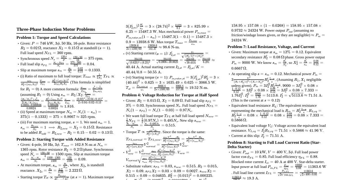
1. Fundamental Equilibrium Condition For any phase equilibrium involving phases $\alpha$ and $\beta$: $\boxed{\mu_i^\alpha = \mu_i^\beta}$ Using fugacity: $\boxed{f_i^\alpha = f_i^\beta}$ This is the universal condition for: VLE (vapor–liquid) LLE (liquid–liquid) VLLE (vapor–liquid–liquid) SLE (solid–liquid) SVE (solid–vapor) Everything else is just models to compute fugacity . 2. Vapor–Liquid Equilibrium (VLE) 2.1 General VLE Equation $f_i^v = f_i^l$ Vapor phase: $f_i^v = y_i \phi_i^v P$ Liquid phase: $f_i^l = x_i \gamma_i f_i^{\text{ref}}$ Often reference state is pure liquid at system T: $f_i^{\text{ref}} = P_i^{sat}\exp\left[\frac{V_i^l (P-P_i^{sat})}{RT}\right]$ Thus: $\boxed{y_i \phi_i P = x_i \gamma_i P_i^{sat}, e^{\frac{V_i^l (P-P_i^{sat})}{RT}} }$ This reduces depending on simplifying assumptions. 2.2 When to use Raoult’s Law Assumptions: Ideal liquid solution: $(\gamma_i = 1)$ Ideal vapor: $(\phi_i = 1)$ Moderate pressures Then: $\boxed{y_i P = x_i P_i^{sat}}$ Use when: Chemically similar components (e.g., benzene–toluene) No strong polarity difference No associating H-bonding mixtures 2.3 When to use Modified Raoult’s Law Used for non-ideal liquid mixtures but still ideal vapor: $\boxed{y_i P = x_i \gamma_i P_i^{sat}}$ Use when: Mixture is moderately non-ideal $\gamma_i$ from Margules, Van Laar, Wilson, NRTL, UNIQUAC Traditional VLE data correlations Examples: Acetone–water Ethanol–water CO$_2$–organics at low pressure 2.4 When to use Henry’s Law For dilute solutes (component i in very small $x_i$): $f_i^l = x_i H_i$ Equilibrium: $y_i P = x_i H_i$ Henry’s law is used when: Solute is sparingly soluble in the solvent System is dilute Component i is not the solvent Typical examples: CO$_2$ in water O$_2$/N$_2$ in water Light gases in organic solvents 3. Liquid–Liquid Equilibrium (LLE) For two immiscible liquid phases $\alpha$ and $\beta$: $\mu_i^\alpha = \mu_i^\beta$ $x_i^\alpha \gamma_i^\alpha = x_i^\beta \gamma_i^\beta$ Key points: Fugacity of each species is equal across phases. No vapor phase condition is used. LLE is determined by: $\boxed{x_i^\alpha \gamma_i^\alpha = x_i^\beta \gamma_i^\beta, i=1..n}$ Physical meaning: $\gamma$ accounts for non-ideality and immiscibility. Use LLE when: Two liquids do not mix well (water–hexane) Temperature is below upper consolute temperature Modeling extraction, decantation, entrainers 4. Vapor–Liquid–Liquid Equilibrium (VLLE) Three phases coexist: vapor + two immiscible liquids. Equilibrium conditions: Vapor–Liquid 1: $f_i^v = f_i^{l1}$ Vapor–Liquid 2: $f_i^v = f_i^{l2}$ Liquid–Liquid: $f_i^{l1} = f_i^{l2}$ Thus all three equal: $\boxed{f_i^v = f_i^{l1} = f_i^{l2}}$ Expanded form: $y_i \phi_i P = x_{i1} \gamma_{i1} f_i^{ref} = x_{i2} \gamma_{i2} f_i^{ref}$ Use VLLE when: Very non-ideal mixtures at low T Alcohol–hydrocarbon systems Refrigerant mixtures Cryogenic systems with immiscibility 5. Solid–Liquid Equilibrium (SLE) General condition: $f_i^s = f_i^l$ Solid phase (pure): $f_i^s = f_i^{s,pure}$ Liquid phase: $f_i^l = x_i \gamma_i f_i^{l,ref}$ Thus: $\boxed{x_i \gamma_i = \frac{f_i^{s,pure}}{f_i^{l,ref}}}$ For melting/freezing point depression: $\ln(x_i \gamma_i) = -\frac{\Delta H_{fus}}{R}\left(\frac{1}{T} - \frac{1}{T_m}\right)$ Use SLE for: Freezing-point depression Eutectic diagrams Crystallization Solubility of solids in liquids 6. Summary Table: When to Use Each Model Problem Type Appropriate Model Conditions Ideal VLE Raoult’s Law Similar molecules, low P Non-ideal VLE Modified Raoult ($\gamma$ models) Strong deviations, azeotropes Gas in liquid (dilute) Henry’s Law Low $x_i$ for solute, sparingly soluble High pressure VLE $\phi–\phi$ EOS method Compressibility high LLE $\gamma$ models only (activity-based) Immiscible liquids VLLE $\gamma–\phi$ for vapor & liquids Multiphase non-ideal systems SLE Solid–liquid fugacity equality Solubility, freezing point 1. Fundamental Condition for Reaction Equilibrium For any reacting system at constant T, P , the equilibrium condition is: $\boxed{\Delta G_{rxn} = 0}$ Or equivalently: $\boxed{\left(\frac{\partial G}{\partial \xi}\right)_{T,P} = 0}$ Where $\xi$ = extent of reaction . The more general statement uses chemical potentials : $\boxed{\sum_i \nu_i \mu_i = 0}$ Where $\nu_i$ = stoichiometric coefficient (products +, reactants −). 2. Equilibrium Constant (K) Definitions The standard definition: $\boxed{K = \exp{\left(-\frac{\Delta G^\circ}{RT}\right)}}$ Important: $(\Delta G^\circ)$ is at standard state (usually 1 bar). 2.1 Gas-Phase Reactions For reaction: $\sum_i \nu_i A_i \rightleftharpoons 0$ General equilibrium expression using fugacity : $\boxed{K = \prod_i \left(\frac{f_i}{f_i^\circ}\right)^{\nu_i}}$ If ideal gas ($f_i = y_i P$): $K = \prod_i (y_i P)^{\nu_i}$ Often separated into: $K = K_p = \prod_i P_i^{\nu_i}$ 2.2 Liquid-Phase Reactions Ideal liquid: $f_i = x_i f_i^\circ$ Then: $K = \prod_i x_i^{\nu_i}$ Non-ideal liquids require activity coefficients: $K = \prod_i (x_i \gamma_i)^{\nu_i}$ 3. Reaction Quotient (Q) For any composition: $Q = \prod_i a_i^{\nu_i}$ Where $(a_i)$ = activity. Comparing Q with K gives direction of shift: Comparison Shift Q Forward reaction Q > K Reverse reaction Q = K At equilibrium 4. Temperature Dependence — van’t Hoff Equation $\boxed{ \frac{d\ln K}{dT} = \frac{\Delta H^\circ}{RT^2} }$ For constant $\Delta H$: $\ln\left(\frac{K_2}{K_1}\right) = -\frac{\Delta H^\circ}{R}\left(\frac{1}{T_2}-\frac{1}{T_1}\right)$ 5. Pressure Effect on Equilibrium For ideal gases: If reaction changes moles of gas: $\Delta n = \sum_i \nu_i$ Increasing pressure favors side with fewer moles of gas . General rule: If $\Delta n forward If $\Delta n > 0$: $\uparrow$P shifts reverse If $\Delta n = 0$: pressure has no effect 6. Extent of Reaction Method (Very Important) Stoichiometric expressions: $n_i = n_{i0} + \nu_i \xi$ Total moles: $n_{tot} = \sum_i n_i$ Mole fractions: $y_i = \frac{n_i}{n_{tot}}$ Plug into equilibrium expression: For ideal gas: $K = \prod (y_i P)^{\nu_i}$ This becomes algebraic equations in terms of $\xi$ . For multiple reactions ($\xi_1, \xi_2\dots$): $n_i = n_{i0} + \sum_j \nu_{i,j} \xi_j$ 7. Common Gas-Phase Equilibrium Expressions 7.1 General ideal-gas form $K = P^{\Delta n} \prod y_i^{\nu_i}$ 7.2 Example: A $\rightleftharpoons$ B + C Stoichiometry: $\nu_A = -1$ $\nu_B = +1$ $\nu_C = +1$ Extent: $n_A = n_{A0} - \xi$ $n_B = n_{B0} + \xi$ $n_C = n_{C0} + \xi$ Total: $n_{tot} = n_0 + \xi$ Mole fractions: $y_A = \frac{n_{A0}-\xi}{n_{tot}}, y_B = \frac{n_{B0}+\xi}{n_{tot}}, y_C = \frac{n_{C0}+\xi}{n_{tot}}$ Equilibrium expression: $K = y_B y_C \frac{P}{y_A}$ Solve for $\xi$. 8. Standard States & Activities Gas Phase Reference state: Ideal gas at 1 bar Activity: $(a_i = f_i/f_i^\circ = y_i \phi_i P / 1,\text{bar})$ Liquid Phase Activity depends on choice: Raoult standard (solvent): ($f_i^\circ = f_i^{pure}$) Henry standard (solute): ($f_i^\circ = H_i$) 9. Multiple Reaction Equilibria For r simultaneous reactions: $n_i = n_{i0} + \sum_{j=1}^r \nu_{ij} \xi_j$ Each reaction provides a K equation. Solve for $\xi_1, \xi_2, \dots, \xi_r$. Used for: Steam methane reforming (SMR + WGS) Cracking reactions Ammonia synthesis with side reactions Combustion equilibrium 10. Reaction Equilibrium with Non-Ideality Gas Nonideality Use fugacity coefficient $\phi_i$: $K = \prod (y_i \phi_i P)^{\nu_i}$ Use EOS (Peng–Robinson, SRK). Liquid Nonideality Use activity coefficient $\gamma_i$: $K = \prod (x_i \gamma_i)^{\nu_i}$ Models: Margules Van Laar Wilson NRTL UNIQUAC 11. Relation Between $\Delta G^\circ, \Delta H^\circ, \Delta S^\circ$ and K $\Delta G^\circ = \Delta H^\circ - T\Delta S^\circ$ $K = e^{-\Delta G^\circ / RT}$ If $\Delta H^\circ > 0$ (endothermic), K $\uparrow$ with T If $\Delta H^\circ K $\downarrow$ with T 12. How to Solve Chemical Equilibrium Problems (Exam Strategy) Step 1 — Write stoichiometric table Include $n_0$, change ($\nu_i \xi$), final $n_i$. Step 2 — Write K expression Use $y_i, x_i$, activities, fugacity as appropriate. Step 3 — Substitute mole fractions Express everything in terms of $\xi$. Step 4 — Solve nonlinear equation(s) Use algebra or numerical solver. Step 5 — Compute final composition Convert moles $\to$ mole fractions. Step 6 — Check Ensure all $n_i \ge 0$, sums = 1. 13. Signs of Stoichiometric Coefficients Role Sign Reactant $-$ (consumed) Product $+$ (formed) This sign convention is essential in $\Delta G$ and equilibrium constant derivations. 14. Special Conditions Equilibrium under constant V (closed rigid container): Minimize Helmholtz free energy: $\left(\frac{\partial A}{\partial \xi}\right)_{T,V}=0$ Equilibrium under constant P (open system): Minimize Gibbs free energy: $\left(\frac{\partial G}{\partial \xi}\right)_{T,P}=0$ 15. Quick Identities to Remember $K = e^{-\Delta G^\circ / RT}$ $\Delta G^\circ = \sum \nu_i G_i^\circ$ $Q = \prod a_i^{\nu_i}$ $K(T) = K(T_0) \exp\left[\frac{\Delta H^\circ}{R}\left(\frac{1}{T_0}-\frac{1}{T}\right)\right]$ Thermodynamic Instability Thermodynamic instability occurs when a mixture cannot minimize its Gibbs free energy by remaining as a single phase. Instead, the mixture lowers its total free energy by splitting into multiple phases (VLE, LLE, SLE, VLLE). This instability is detected using criteria based on chemical potentials , Gibbs energy curvature , and tangent-plane stability tests . 1. Fundamental Stability Requirement At constant T and P , a single-phase mixture is stable only if: $\boxed{\left( \frac{\partial^2 G}{\partial n_i \partial n_j} \right)_{T,P} \text{ is positive semidefinite}}$ In simpler terms: The Gibbs free energy as a function of composition must be convex. If the mixture Gibbs free energy curve becomes concave (curvature 2. Mathematical Condition for Instability For a binary mixture: Let $g(x_1) = \frac{G}{n}$ Thermodynamic stability requires: $\boxed{\frac{d^2 g}{dx_1^2} \ge 0}$ If: $\frac{d^2 g}{dx_1^2} $\to$ Mixture is unstable $\to$ Phase splitting occurs $\to$ Typically results in LLE or VLLE . 3. Physical Meaning (Very Important) If G vs. composition curve bends upward $\to$ stable one phase If it bends downward $\to$ unstable $\to$ splits If it has two minima $\to$ two-phase region This is the basis of the common tangent rule . 4. Common Tangent Condition (Phase Splitting) For phase $\alpha$ and phase $\beta$: $g^\alpha(x_1^\alpha) = g^\beta(x_1^\beta)$ and the slope is the same: $\left(\frac{dg}{dx_1}\right)_{x^\alpha} = \left(\frac{dg}{dx_1}\right)_{x^\beta}$ If such a tangent exists, the mixture is unstable in the composition range: $x_1^\alpha 5. Spinodal Region (Inside the LLE Envelope) The spinodal defines complete instability . Condition: $\frac{d^2 g}{dx_1^2} = 0$ Regions: Stable region : $(\frac{d^2 g}{dx_1^2} > 0)$ Metastable region (nucleation required): Still convex but above the common tangent Unstable region (spinodal): $(\frac{d^2 g}{dx_1^2} In spinodal region, even infinitesimal fluctuations lead to phase separation . 6. Conditions for VLE, LLE, VLLE Based on Stability VLE (Vapor–Liquid Equilibrium) Occurs when vapor and liquid satisfy: $f_i^v = f_i^l$ Instability occurs if: $G_{mixture} > G_{two-phase}$ LLE (Liquid–Liquid Equilibrium) Occurs when two immiscible liquids satisfy: $f_i^\alpha = f_i^\beta$ Instability $\to$ double-well Gibbs energy curve $\to$ Two minima. VLLE (Vapor–Liquid–Liquid Equilibrium) Occurs when: $f_i^v = f_i^\alpha = f_i^\beta$ This requires: A vapor phase stable Two distinct liquid phases with equal tangent-plane slopes All three satisfy equilibrium fugacity conditions VLLE appears only when mixture exhibits deep liquid–liquid immiscibility and strong non-ideality . 7. Tangent Plane Distance (TPD) Stability Test General test used in advanced thermodynamics (EOS-based): For trial composition ($w_i$): $TPD(w) = \sum_i w_i \left[ \ln w_i + \ln \phi_i(w) - \ln z_i - \ln \phi_i(z) \right]$ If: $TPD(w) \ge 0 \quad \forall w$ Mixture is stable . If: $TPD(w) Mixture is unstable $\to$ phase split must occur. 8. Summary of Instability Conditions Condition Meaning Phase Result $(\frac{d^2 g}{dx^2} > 0)$ Stable mixture 1 phase $(\frac{d^2 g}{dx^2} = 0)$ Spinodal Onset of instability $(\frac{d^2 g}{dx^2} Unstable Must split into phases Common tangent exists Two-phase lower G LLE or VLLE TPD Unstable Split according to EOS 9. Why Thermodynamic Instability Happens Common causes: A. Strongly non-ideal mixtures ($\gamma \gg 1$) $\to$ often water–organic systems. B. Large solubility parameter differences (regular solution theory): $g^E \propto (\delta_1 - \delta_2)^2$ C. Temperature change Cooling often induces: LLE Solid–liquid separation Crystallization D. Pressure change High pressure can promote VLLE. 10. Diagrams Used to Diagnose Instability A. Gibbs free energy vs. composition plot Shows convex/concave regions. B. Phase diagram (binodal + spinodal) Outer curve = binodal (LLE boundary) Inner curve = spinodal (complete instability) C. Tangent-plane distance plots Used in EOS-phase stability.