Linear Models Cheatsheet
Cheatsheet Content
### Matrix Theory Review #### Matrix A matrix is a rectangular array of numbers, symbols, or expressions organized into rows and columns. $$ A = \begin{bmatrix} 1 & 2 & 3 \\ 4 & 5 & 6 \\ 7 & 8 & 9 \end{bmatrix}, B = \begin{bmatrix} 10 & 11 & 12 \\ 7 & 82 & 19 \end{bmatrix} $$ #### Vector A vector is an array of numbers arranged in a row or column. $$ \vec{a} = \begin{bmatrix} 1 \\ 2 \\ 3 \end{bmatrix}, \vec{a}' = \begin{bmatrix} 1 & 2 & 3 \end{bmatrix} $$ #### Scalar A single number. Example: $a = 1$ #### Property of Matrices: Equality Two matrices are equal if they have the same dimensions and corresponding elements. $$ A = \begin{bmatrix} a & b & c \\ d & e & f \\ g & h & i \end{bmatrix}, B = \begin{bmatrix} a & b & c \\ d & e & f \\ g & h & i \end{bmatrix} \implies A = B $$ #### Property of Matrices: Transpose A transpose of a matrix ($A^T$ or $A'$) is formed by interchanging rows and columns. If $A = \begin{bmatrix} 1 & 2 \\ 3 & 4 \end{bmatrix}$, then $A^T = A' = \begin{bmatrix} 1 & 3 \\ 2 & 4 \end{bmatrix}$ #### Property of Matrices: Symmetry A matrix is symmetric if it is equal to its own transpose ($A^T = A$). If $A = \begin{bmatrix} 3 & 5 \\ 5 & 3 \end{bmatrix}$, then $A^T = \begin{bmatrix} 3 & 5 \\ 5 & 3 \end{bmatrix}$, so $A^T = A$. #### Property of Matrices: Sum and Difference The sum or difference of two matrices of the same order is obtained by performing addition or subtraction on their corresponding elements. $$ A = \begin{bmatrix} 1 & 4 & 0 \\ 5 & 1 & 5 \\ 7 & 3 & 2 \end{bmatrix}, B = \begin{bmatrix} 2 & 2 & 2 \\ 3 & 1 & 5 \\ 1 & 6 & 8 \end{bmatrix} $$ $A+B = \begin{bmatrix} 3 & 6 & 2 \\ 8 & 2 & 10 \\ 8 & 9 & 10 \end{bmatrix}$, $B-A = \begin{bmatrix} 1 & -2 & 2 \\ -2 & 0 & 0 \\ -6 & 3 & 6 \end{bmatrix}$ #### Property of Matrices: Multiplication Matrix multiplication is applicable to conformable matrices. If $A = [a_{ij}]_{m \times n}$ and $B = [b_{jk}]_{n \times p}$, then the product $C = A \cdot B$ is: $$ c_{ij} = \sum_{k=1}^{n} a_{ik}b_{kj} $$ #### Special Type: Identity Matrix The identity matrix ($I$) is a square matrix with 1's on the main diagonal and 0's elsewhere. $$ I = \begin{bmatrix} 1 & 0 & \dots & 0 \\ 0 & 1 & \dots & 0 \\ \vdots & \vdots & \ddots & \vdots \\ 0 & 0 & \dots & 1 \end{bmatrix} $$ #### Orthogonal Vectors Orthogonal vectors are perpendicular to each other. They are linearly independent (unless one is the zero vector). If $\vec{a}$ and $\vec{b}$ are vectors and $\vec{a}^T\vec{b} = \vec{b}^T\vec{a} = 0$, then $\vec{a}$ is orthogonal to $\vec{b}$. #### Inverse of a Matrix The inverse of a matrix $A^{-1}$ is a matrix that, when multiplied by $A$, gives the identity matrix $I$. It exists only if $A$ is square and non-singular ($\det(A) \neq 0$). $$ A^{-1}A = I = AA^{-1} $$ If $A\vec{x} = \vec{y}$ then $\vec{x} = A^{-1}\vec{y}$ if $A$ is non-singular. #### Linear Dependence Supposed $A = \{\vec{v}_1, \vec{v}_2, ..., \vec{v}_n\}$ is linearly dependent if there exist scalars $c_1, c_2, ..., c_n$, not all zero, such that: $$ c_1\vec{v}_1 + c_2\vec{v}_2 + \dots + c_n\vec{v}_n = 0 $$ If the only solution is all $c_i = 0$, then the vectors are linearly independent. #### Singular Matrix A singular matrix is a square matrix that does not have an inverse. This happens when its determinant equals zero. A matrix whose rows or columns are linearly dependent is singular. #### Determinant A scalar value summarizing a matrix. - For a $2 \times 2$ matrix $A = \begin{bmatrix} a & b \\ c & d \end{bmatrix}$, the determinant is $|A| = ad - bc$. - For a $3 \times 3$ matrix $A = \begin{bmatrix} a & b & c \\ d & e & f \\ g & h & i \end{bmatrix}$, the determinant is $|A| = aei + bfg + cdh - ceg - afh - bdi$. #### Rank The rank of a matrix $\text{rank}(A)$ is the number of linearly independent rows or columns in the matrix. #### Trace The trace of a matrix is the sum of the elements on its main diagonal (from top-left to bottom-right). If $A = \{a_{ij}\}$, $i,j = 1, ..., n$, then $$ \text{tr}(A) = \sum_{i=1}^{n} a_{ii} $$ Properties: - $\text{tr}(A+B) = \text{tr}(A) + \text{tr}(B)$ - $\text{tr}(AB) = \text{tr}(BA)$ - $\text{tr}(ABC) = \text{tr}(CAB) = \text{tr}(BCA)$ #### Characteristic Equation The characteristic equation of a matrix is the polynomial equation obtained from its determinant, used to find the matrix's eigenvalues. $$ \det(A - \lambda I) = 0 $$ This is an $n^{th}$ degree polynomial, implying $n$ possible solutions for $\lambda$. #### Eigenvalues & Eigenvectors - **Eigenvalues ($\lambda_i$):** The solutions to the characteristic equation. - **Eigenvectors ($\vec{v}_i$):** For each eigenvalue $\lambda_i$, the solution to the system $A\vec{v}_i = \lambda_i\vec{v}_i$ is the eigenvector associated with $\lambda_i$. ### Introduction to Linear Regression #### Variables and Data Types - **Variables:** Fundamental concepts representing characteristics or properties that can take on different values. - **Dependent Variables (DV):** The outcome we're trying to predict (response variable). - **Independent Variables (IV):** Predictor variables that influence changes in the dependent variable. - **Identifying Research Variables:** Crucial first step in linear regression analysis. - **Data Types:** - **Time-Series Data:** Measurements taken over time (e.g., monthly stock prices). - **Cross-Sectional Data:** Measurements taken at a single point in time (e.g., survey data on income). #### Classification of Linear Models and the Model Building Process - **General Classification:** - **Structural models:** Explain variability of the variable of interest using other variables. - **Nonstructural models:** Explain variability of a variable using past values or observations. - **The Model Building Process:** - **Model:** A set of assumptions summarizing a system's structure. - **Purpose of Modeling:** Understand data generation mechanism, predict DV values given IVs, optimize response. - **Process Steps:** 1. **Planning:** Define research question, identify variables, select data sources. 2. **Development:** Choose appropriate model, fit to data, select relevant IVs, estimate coefficients, assess fit. 3. **Verification and Maintenance:** Evaluate performance, identify biases, update model as needed. - **Goal:** Create an accurate and interpretable model. #### Regression Analysis - **Historical Origin:** Dates back to 19th-century Sir Francis Galton's work on heredity, where "regression towards mediocrity" described the tendency of extreme values to move towards the average. - **The Linear Model:** - Slope-intercept form of a line: $Y = mX + b$, where $b$ is the Y-intercept and $m$ is the slope. - For $n$ samples, $(X_i, Y_i)$: - Straight line: $Y = \beta_0 + \beta_1X$ - Each point: $Y_i = \beta_0 + \beta_1X_i + \epsilon_i$ - With $k$ independent variables: $Y_i = \beta_0 + \beta_1X_{i1} + \beta_2X_{i2} + \dots + \beta_kX_{ik} + \epsilon_i$ - $\beta$'s are parameters, $\epsilon$'s are error terms. - **Why include error terms?** 1. **Measurement errors:** Inaccuracies in DV or IV measurements. 2. **Other IVs not included:** Relevant factors affecting DV not in the model. 3. **Unexplained variability in Y:** Variability remaining even after accounting for all relevant IVs. - Error terms allow for realistic modeling, acknowledge messy real-world data, and maintain integrity of predictions. #### Assumptions of Linear Regression Model - **Purpose of Assumptions:** Regulate the balance between summarizing sample data and model fit. - **Classical Assumptions (about error terms $\epsilon_i$):** 1. Expected value of error is zero: $E(\epsilon_i) = 0$ 2. Constant variance (homoscedasticity): $\text{Var}(\epsilon_i) = \sigma^2$ 3. Errors are uncorrelated: $\text{Cov}(\epsilon_i, \epsilon_j) = 0$, for $i \neq j$ - **Other Assumptions:** 1. **Normal error Model Assumption:** $\epsilon_i \sim N(0, \sigma^2)$ (Independently and identically distributed). 2. Independent Variables are predetermined and uncorrelated. 3. Dependent variables follow $N(X\beta, \sigma^2 I)$. - **Important Note:** Assumptions about the distribution are on the error terms, not on the dependent variable. ### Model Summary & Analysis of Variance #### Review of Some Notations | Notation | Definition | |----------|------------| | $X, \vec{X}$ | Vector of predictor variable values (predetermined). | | $Y, \vec{Y}$ | Vector of observed dependent variable values. | | $\bar{Y}$ | Mean or average of observed values. | | $\beta, \vec{\beta}$ | Vector of coefficients (parameters) in the regression model. | | $\epsilon$ | Inherent variability: true differences between observed values and true model values ($Y_i - \mu_i$). | | $e$ | Assesses model fit/validity: differences between observed and predicted values from the model ($Y_i - \hat{Y}_i$). | #### Multiple Linear Regression in Matrix Form For $n$ samples with $k$ independent variables: $$ \vec{Y} = X\vec{\beta} + \vec{\epsilon} $$ $$ \begin{bmatrix} Y_1 \\ Y_2 \\ \vdots \\ Y_n \end{bmatrix} = \begin{bmatrix} 1 & X_{11} & X_{12} & \dots & X_{1k} \\ 1 & X_{21} & X_{22} & \dots & X_{2k} \\ \vdots & \vdots & \vdots & \ddots & \vdots \\ 1 & X_{n1} & X_{n2} & \dots & X_{nk} \end{bmatrix} \begin{bmatrix} \beta_0 \\ \beta_1 \\ \vdots \\ \beta_k \end{bmatrix} + \begin{bmatrix} \epsilon_1 \\ \epsilon_2 \\ \vdots \\ \epsilon_n \end{bmatrix} $$ - For predicted values: $\hat{Y} = X\hat{\beta}$ #### The Least Squares Theory - **Goal:** Estimate model coefficients by minimizing the sum of squared differences (residuals) between observed values and predicted values. This is known as the sum of squared errors (SSE). - **Least Squares Estimator for $\vec{\beta}$:** $$ \hat{\vec{\beta}} = (X^T X)^{-1} X^T \vec{Y} $$ - **Fitted Values of $\vec{Y}$:** $$ \hat{\vec{Y}} = X\hat{\vec{\beta}} = X(X^T X)^{-1} X^T \vec{Y} $$ - **Residuals ($e$):** $$ \vec{e} = \vec{Y} - \hat{\vec{Y}} = \vec{Y} - X\hat{\vec{\beta}} = \vec{Y} - X(X^T X)^{-1} X^T \vec{Y} = (I - X(X^T X)^{-1} X^T) \vec{Y} = (I - H)\vec{Y} $$ Where $H = X(X^T X)^{-1} X^T$ is the *hat matrix*. Also, $\hat{\vec{\beta}} = \vec{\beta} + (X^T X)^{-1} X^T \vec{\epsilon}$. The vector of residuals is a null vector. #### Inferences in Regression Analysis - Analysis of Variance - **Purpose:** Evaluate if the model explains variation in Y based on X variables. ANOVA helps determine how well the regression model explains variability by comparing variance explained by the model to unexplained residual variance. - **Sum of Squares (SS):** - **SST (Total Sum of Squares):** Total variability in Y. $$ \text{SST} = \sum_{i=1}^{n} (Y_i - \bar{Y})^2 = (\vec{Y} - \bar{Y}\vec{1})^T (\vec{Y} - \bar{Y}\vec{1}) $$ - **SSR (Sum of Squares Regression):** Variation in Y explained by the model. $$ \text{SSR} = \sum_{i=1}^{n} (\hat{Y}_i - \bar{Y})^2 = (\hat{\vec{Y}} - \bar{Y}\vec{1})^T (\hat{\vec{Y}} - \bar{Y}\vec{1}) $$ - **SSE (Sum of Squares Error):** Unexplained variation in Y (residual variation). $$ \text{SSE} = \sum_{i=1}^{n} (Y_i - \hat{Y}_i)^2 = \vec{e}^T\vec{e} $$ - **Degrees of Freedom (df):** - SST has df of $n-1$. - SSR has df of $p-1$ (where $p = k+1$ for $k$ predictors and intercept). - SSE has df of $n-p$. - **Mean Squares (MS):** Average of squared deviations, used to estimate variance components and for hypothesis testing. - **MSR (Mean Square Regression):** $\text{MSR} = \frac{\text{SSR}}{p-1}$ - **MSE (Mean Square Error):** $\text{MSE} = \frac{\text{SSE}}{n-p}$ - **Hypothesis Testing involving ANOVA:** - Null Hypothesis ($H_0$): $\beta_0 = \beta_1 = \beta_2 = \dots = \beta_k = 0$ (all slopes are zero, model has no explanatory power). - Alternative Hypothesis ($H_a$): At least one $\beta_j \neq 0$. - **F-statistic:** $$ F_{\text{stat}} = \frac{\text{MSR}}{\text{MSE}} \sim F_{(p-1, n-p)} $$ - **Rejection Criteria:** Reject $H_0$ if $F_{\text{stat}} > F_{\alpha, p-1, n-p}$ or if $p$-value ### Regression Coefficients & Model Summary #### Unstandardized Coefficients - Represent the actual change in the dependent variable for a one-unit change in the independent variable, holding all other variables constant. - Example: $\hat{Y} = 97.26 + 0.304X_1 + 0.122X_2 - 0.038X_3 + 0.345X_4$ - For every 1 unit increase in $X_1$, $\hat{Y}$ increases by 0.304 units. - For every 1 unit increase in $X_3$, $\hat{Y}$ decreases by 0.038 units. #### Standard Error of Coefficients - Indicates the average distance the estimated coefficients are expected to be from the actual population parameter. - A smaller standard error suggests greater precision. #### t-Value Used to conduct hypothesis tests to see if each coefficient is significantly different from zero. $$ t = \frac{\text{Coefficient}}{\text{Standard Error}} $$ - Compare $t$-value against critical values from a $t$-distribution with $df = n-k-1$. - Alternatively, check if $p$-value (Sig. column) #### Standardized Coefficients (Beta Weights) - Used to understand the relative importance of each predictor variable. - Calculated by converting raw scores of DV and IVs into z-scores (mean 0, std dev 1). - Allow direct comparison of effect strength across different predictors (same scale). - A higher absolute value indicates a stronger effect. - Indicates how many standard deviations the dependent variable will change for a one-standard-deviation change in the predictor variable. #### Model Summary - **R (Correlation):** Degree of correlation between all IVs and the DV. - **R Square ($R^2$):** Proportion of total variation in the DV explained by the IVs. $$ R^2 = \frac{\text{SSR}(X_1, X_2, \dots, X_k)}{\text{SST}} = 1 - \frac{\text{SSE}(X_1, X_2, \dots, X_k)}{\text{SST}} $$ - Lies between 0 and 1. If $k=1$, $R^2 = r^2$. - Caution: High $R^2$ doesn't necessarily mean a good fit or useful prediction. Correlation doesn't imply causation. - **Coefficient of Alienation (D):** Proportion of variability in the dependent variable *not* explained by the independent variable(s). $$ D = 1 - R^2 $$ - **Adjusted R-Squared:** Modified $R^2$ accounting for the number of predictors. Provides a more accurate measure of how well the model explains variability, especially with multiple IVs. $$ R^2_{\text{adj}} = 1 - \frac{\text{MSE}}{\text{MST}} = 1 - \frac{\text{SSE}/(n-p)}{\text{SST}/(n-1)} $$ - An increase in Adjusted $R^2$ suggests improved fit. If it decreases when adding predictors, it indicates potential overfitting. - **Standard Error of the Estimate:** Standard deviation of the errors/residuals. ### Confidence Intervals & Prediction #### Gauss-Markov Theorem - Under MLR model conditions ($E(\epsilon) = 0$, $\text{Var}(\epsilon) = \sigma^2I$), the least squares estimator $\hat{\beta}$ is the **Best Linear Unbiased Estimator (BLUE)** of $\beta$. - This means $\hat{\beta}$ has the smallest variance among all linear unbiased estimators. - Furthermore, any linear combination $\lambda^T\hat{\beta}$ of the elements of $\hat{\beta}$ is BLUE. - With normality assumption, $\hat{\beta}$ and $\hat{\sigma}^2 = \vec{e}^T\vec{e}/(n-p)$ are maximum likelihood estimators (MLEs). - $(\hat{\beta}, \hat{\sigma}^2)$ is the UMVUE (Uniformly Minimum Variance Unbiased Estimator) for $(\beta, \sigma^2)$. #### Confidence Intervals (CI) - Provide a range of values within which we expect the true population parameter (e.g., slope, intercept) to lie, with a certain level of confidence (commonly 95%). - For coefficients: $$ \hat{\beta}_j \pm t_{\alpha/2, (n-p)} \cdot SE(\hat{\beta}_j) $$ - **Confidence Ellipsoid:** Used for joint confidence regions for multiple parameters. $$ \frac{(\hat{\vec{\beta}} - \vec{\beta})^T X^T X (\hat{\vec{\beta}} - \vec{\beta})}{p \cdot \hat{\sigma}^2} \sim F_{(p, n-p)} $$ #### Prediction Intervals (PI) - Provide a range of values likely to contain the value of a *new observation*. - Account for both uncertainty in estimated coefficients and variability of individual observations. - Formula for a new observation $\hat{Y}_{\text{new}}$: $$ \hat{Y}_{\text{new}} \pm t \cdot SE_{\text{pred}} $$ where $\hat{Y}_{\text{new}}$ is the predicted value, $t$ is the critical value, and $SE_{\text{pred}}$ is the standard error of the prediction. - **Standard Error of the Prediction:** Includes error of estimate and variability of response. $$ SE_{\text{pred}} = \sqrt{SE^2 + \sigma^2} $$ - $SE$ is standard error of predicted mean response. - $\sigma^2$ is variance of residuals. - **Reminders:** PIs are typically wider than CIs because they account for both model uncertainty and natural data variability. Useful for forecasting. #### Inverse Regression Problem (Calibration Problem) - Involves estimating the relationship between dependent and independent variables, but from the perspective of predicting the *independent variables given the dependent variables*. - Focuses on how changes in the DV inform or predict changes in the IVs. - Useful when DV measurements are more reliable than IVs. Requires different techniques and assumptions than standard regression.