Analytical Chemistry Intro

Cheatsheet Content

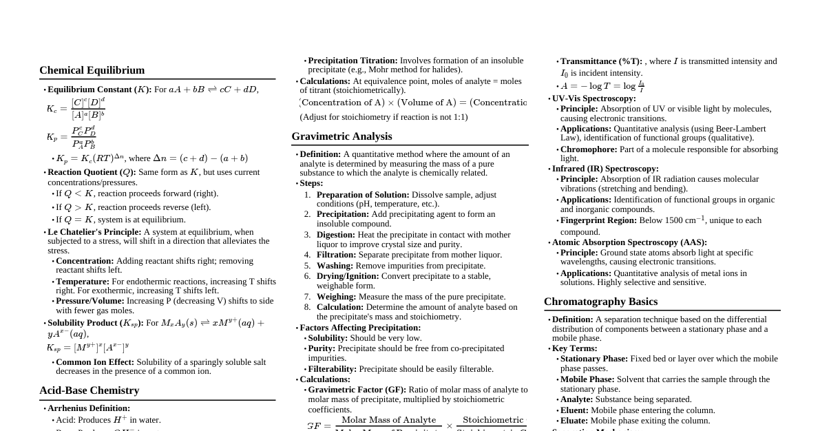
### Introduction to Analytical Chemistry Analytical chemistry involves the chemical characterization of sample materials. - **Analyte**: The component of a sample to be determined. - **Matrix**: All substances in the sample except the analyte. #### Scope and Role Analytical chemistry plays a crucial role in various fields: - **Forensic**: Provides chemical evidence. - **Manufacturing**: Ensures quality control of products like food and drugs. - **Environmental**: Supports sustainability and protection of natural resources. - **Purpose**: To gather and interpret chemical information valuable to society. ### General Terms in Chemical Analysis #### Sample-Related Terms - **Sample**: A representative portion of the tested material (e.g., soil sample). - **Analyte**: The specific substance being measured (e.g., cholesterol). - **Matrix**: All other substances in the sample apart from the analyte. #### Method-Related Terms - **Method (Assay/Analysis/Determination)**: The overall approach to characterize a sample (e.g., hemoglobin analysis). - **Analytical Technique**: The specific approach used to perform an assay (e.g., spectroscopy, filtration). - **Procedure/Protocol**: The entire sequence of operations for an analysis. ### Types of Quantitative Analysis 1. **Classical Methods**: - **Gravimetric Analysis**: Based on determining the mass of a pure compound related to the analyte (e.g., determining sulfate by precipitating as BaSO₄). - **Volumetric Analysis**: Based on measuring the volume of a reagent of known concentration that reacts completely with the analyte (e.g., complexometric titration for water hardness). 2. **Instrumental Methods**: Utilize instruments for analysis (e.g., Spectroscopy, Electrochemistry, Chromatography). 3. **Coupled Methods**: Combine multiple techniques. #### Extent of Analysis - **Ultimate**: Very detailed characterization. - **Proximate**: Less detailed, focuses on groups of components. #### Sample Size - **Macro**: >100 mg or >100 µL - **Semi-micro**: 10-100 mg or 50-100 µL - **Micro**: 1-10 mg or 1% - **Minor**: 0.01% - 1% - **Trace**: 1 ppb - 0.01% - **Ultratrace**: ### Steps in Quantitative Analysis 1. **Plan**: - Define the problem and information needed. - Choose an analytical method considering accuracy, precision, time, cost, and sample complexity. 2. **Sampling**: - Identify the population. - Obtain a gross sample (representative of the population). - Obtain a laboratory sample (smaller portion for analysis). 3. **Sample Preparation**: - Homogenize the sample. - Convert to a suitable form for analysis. - Avoid decomposition. - Eliminate interferences. - Define replicate samples (portions carried through analysis identically). 4. **Analytical Measurement**: Determine analyte concentration (direct or indirect). 5. **Data Analysis**: Calculate and evaluate results. ### Measures of Central Tendency and Spread Measurements invariably involve errors. Replicates improve reliability and provide information about variability. #### Central Tendency (Best Estimate of True Value) - **Mean ($\bar{x}$)**: Average of $N$ replicates. $$\bar{x} = \frac{\sum x_i}{N}$$ - **Median ($x_{med}$)**: Middle value of an ordered data set. Less sensitive to outliers. - **Mode**: Most frequent result. #### Spread (Estimates Variability) - **Range ($w$)**: Difference between largest and smallest values ($w = X_{largest} - X_{smallest}$). - **Deviation ($d_i$)**: Difference of an individual measurement from the mean ($d_i = x_i - \bar{x}$). - **Average Deviation ($\bar{d}$)**: Average of absolute deviations ($ \bar{d} = \frac{\sum |d_i|}{N}$). - **Standard Deviation ($s$)**: Describes spread of individual measurements about the mean. $$s = \sqrt{\frac{\sum (x_i - \bar{x})^2}{N-1}}$$ - **Variance ($s^2$)**: Square of the standard deviation. - **Relative Standard Deviation (RSD)**: $$RSD = \frac{s}{\bar{x}}$$ - Often expressed as parts per thousand or percent. - **Coefficient of Variation (CV)**: $CV = RSD \times 100\%$. ### Characterizing Experimental Errors #### Accuracy - Measure of how close a measurement is to the true value ($\mu$). - **Absolute Error ($E$)**: $E = \bar{x} - \mu$ - Positive if $\bar{x} > \mu$, negative if $\bar{x} ### Types of Errors in Experimental Data 1. **Systematic Errors (Determinate Errors)**: - Affects **accuracy**. - Results are usually constant in both magnitude and direction. - Can be determined and eliminated/corrected. - Sources: - **Instrumental errors**: Faulty calibration, non-ideal instrument behavior. - **Method errors**: Non-ideal chemical/physical behavior of analytical systems. - **Personal errors**: Carelessness, personal limitations. - **Sampling errors**: Fails to provide a representative sample. - Effects: - **Constant errors**: Independent of sample size. - **Proportional errors**: Increase/decrease in proportion to sample size. - Detection: Periodic calibration, analysis of standard samples, independent analysis, blank determinations. 2. **Random Errors (Indeterminate Errors)**: - Affects **precision**. - Has an equal chance of being positive or negative. - Cannot be eliminated, but can be minimized by increasing the number of trials. - Sources: Small, undetectable uncertainties in sample collection, manipulation, and measurement. 3. **Gross Errors**: - Affects **accuracy**. - Leads to **outliers** (results significantly different from the rest). - Can be determined and eliminated/corrected. ### Propagation of Errors The uncertainty (standard deviation, $s$) in each measurement accumulates. #### For Addition and Subtraction If $a = b + c - d$, then the absolute variance of $a$ is the sum of the absolute variances of each measurement: $$s_a^2 = s_b^2 + s_c^2 + s_d^2$$ $$s_a = \sqrt{s_b^2 + s_c^2 + s_d^2}$$ #### For Multiplication and Division If $a = \frac{bc}{d}$, then the relative variance of $a$ is the sum of the relative variances of each measurement: $$\left(\frac{s_a}{a}\right)^2 = \left(\frac{s_b}{b}\right)^2 + \left(\frac{s_c}{c}\right)^2 + \left(\frac{s_d}{d}\right)^2$$ $$s_{a,rel} = \sqrt{s_{b,rel}^2 + s_{c,rel}^2 + s_{d,rel}^2}$$ $$s_a = a \times s_{a,rel}$$ #### For Powers If $a = b^x$, then $\frac{s_a}{a} = x \frac{s_b}{b}$. Example: If $s = K_{sp}^{1/2}$, then $\frac{s_s}{s} = \frac{1}{2}\frac{s_{K_{sp}}}{K_{sp}}$. ### Confidence Interval (CI) The CI describes the variability of a data set, representing the range within which the true mean ($\mu$) is expected to lie with a certain probability. - **Confidence Interval**: Range of values for $\mu$. - **Confidence Limits**: Boundaries of the CI (e.g., $2.2 \text{ ppm}$ to $2.8 \text{ ppm}$). - **Confidence Level**: Probability that the true mean lies within the interval (e.g., 90%). - **Significance Level ($\alpha$)**: Probability that the result is outside the CI (e.g., 10% for 90% confidence). #### CI when Population Standard Deviation ($\sigma$) is Known (or $s$ is a good estimate of $\sigma$) $$CI = \bar{x} \pm z \frac{\sigma}{\sqrt{N}}$$ where $z$ is obtained from the z-table for the given confidence level. #### CI when Population Standard Deviation ($\sigma$) is Unknown Use the Student's t-distribution: $$CI = \bar{x} \pm t \frac{s}{\sqrt{N}}$$ where $t$ is obtained from the t-table for the given confidence level and degrees of freedom ($df = N-1$). - **Degrees of Freedom ($df$)**: Number of members in a sample that provide an independent measure of precision. ### Statistical Analysis Hypothesis tests determine if experimental results support a model. - **Null Hypothesis ($H_0$)**: Assumes numerical quantities are statistically the same. - **Alternative Hypothesis ($H_a$)**: Assumes numerical quantities are significantly different. #### Test Procedure 1. **Formulate a test statistic**. 2. **Identify a rejection region**. If the calculated test statistic falls within this region, $H_0$ is rejected. #### Common Statistical Tests 1. **Comparing a Mean to a Reference Value ($\mu_0$) (t-test)** - Used when $\sigma$ is unknown. - $H_0: \bar{x} = \mu_0$ - $H_a: \bar{x} \neq \mu_0$ (two-tailed) or $H_a: \bar{x} > \mu_0$ or $H_a: \bar{x} t_{crit}$, reject $H_0$. 2. **Comparison of Variances (F-test)** - Used to compare precision of two methods/sets of data. - $H_0: s_1^2 = s_2^2$ - $H_a: s_1^2 > s_2^2$ (one-tailed) or $H_a: s_1^2 \neq s_2^2$ (two-tailed) $$F_{calc} = \frac{s_1^2}{s_2^2}$$ - Always place the larger variance in the numerator ($s_1^2 > s_2^2$). - Compare $F_{calc}$ with $F_{crit}$ (from F-table, $df_1 = N_1-1$, $df_2 = N_2-1$). - If $F_{calc} > F_{crit}$, reject $H_0$. 3. **Comparison of Two Experimental Means (t-test)** - Used to determine if two means are significantly different. - F-test should be done first to ensure variances are similar. - $H_0: \bar{x}_1 = \bar{x}_2$ - $H_a: \bar{x}_1 \neq \bar{x}_2$ $$t_{calc} = \frac{|\bar{x}_1 - \bar{x}_2|}{s_{pooled} \sqrt{\frac{1}{N_1} + \frac{1}{N_2}}}$$ $$s_{pooled} = \sqrt{\frac{(N_1-1)s_1^2 + (N_2-1)s_2^2}{N_1+N_2-2}}$$ - Compare $t_{calc}$ with $t_{crit}$ (from t-table, $df = N_1+N_2-2$). - If $|t_{calc}| > t_{crit}$, reject $H_0$. 4. **Paired Data (t-test)** - Used when measurements are collected in pairs (e.g., same sample analyzed by two methods) to eliminate variability. - $H_0: \bar{d} = \Delta_0$ (often $\Delta_0 = 0$) - $H_a: \bar{d} \neq \Delta_0$ $$t_{calc} = \frac{\bar{d} - \Delta_0}{s_d/\sqrt{N}}$$ where $\bar{d}$ is the average difference, and $s_d$ is the standard deviation of the differences. - Compare $t_{calc}$ with $t_{crit}$ (from t-table, $df = N-1$, where $N$ is the number of pairs). - If $|t_{calc}| > t_{crit}$, reject $H_0$. 5. **Outlier Tests** - Used to identify and potentially remove gross errors (outliers). - **Dixon's Q-test**: $$Q_{calc} = \frac{|x_{suspect} - x_{nearest}|}{x_{range}}$$ - Compare $Q_{calc}$ with $Q_{crit}$. If $Q_{calc} > Q_{crit}$, reject the suspected value. - **Grubb's test**: $$G_{calc} = \frac{|x_{suspect} - \bar{x}|}{s}$$ - Compare $G_{calc}$ with $G_{crit}$. If $G_{calc} > G_{crit}$, reject the suspected value. - If an outlier is rejected, recalculate mean, standard deviation, and re-test. ### Review of Concepts of Stoichiometry: Mole Concept - **Mole**: Fundamental quantity representing the amount of matter. $1 \text{ mole} = 6.022 \times 10^{23}$ particles (Avogadro's number). - **Atomic Mass/Weight**: Mass of one mole of an element (g/mol), found on the periodic table. - **Molecular Mass/Weight**: Mass of one mole of a compound (g/mol). Sum of atomic masses of all atoms in the formula. - **Molar Mass (MM)**: The mass in grams of one mole of a substance. #### Conversions - **Mass to Moles**: $$\text{moles} = \frac{\text{mass (g)}}{\text{MM (g/mol)}}$$ - **Moles to Mass**: $$\text{mass (g)} = \text{moles} \times \text{MM (g/mol)}$$ - **Moles to Number of Particles**: $$\text{Number of Particles} = \text{moles} \times (6.022 \times 10^{23} \text{ particles/mol})$$ - Particles can be atoms (for elements), molecules (for covalent compounds), formula units (for ionic compounds), or ions. ### Review of Concepts of Stoichiometry: Percent Composition, Empirical and Molecular Formulas #### Percent Composition - The mass percentage of each element in a compound. $$\% \text{ Element} = \frac{(\text{Number of atoms of element}) \times (\text{Atomic mass of element})}{\text{Molecular mass of compound}} \times 100\%$$ #### Empirical Formula - The simplest whole-number ratio of atoms in a compound. - **Steps to derive**: 1. Assume a 100 g sample (convert % to grams). 2. Convert grams of each element to moles using atomic mass. 3. Divide all mole values by the smallest mole value to get initial ratios. 4. If ratios are not whole numbers, multiply by a common factor to get whole numbers. #### Molecular Formula - The actual number of atoms of each element in a molecule. - **Steps to derive (from empirical formula)**: 1. Calculate the empirical formula mass (EFM). 2. Determine the integer factor ($n$): $$n = \frac{\text{Molecular Mass}}{\text{Empirical Formula Mass}}$$ 3. Multiply the subscripts in the empirical formula by $n$. ### Review of Concepts of Stoichiometry: Stoichiometry Stoichiometry refers to the quantitative aspects of chemical composition and reactions. #### Balancing Chemical Reactions 1. **Write correct formulas**: Ensure names are converted to correct chemical formulas. Remember diatomic elements (H₂, N₂, O₂, F₂, Cl₂, Br₂, I₂). 2. **Count atoms**: Sum atoms of each element on reactant and product sides. 3. **Adjust coefficients**: Change coefficients (numbers preceding chemical species) to balance elements. **Never change subscripts**. 4. **Simplify coefficients**: Reduce to the lowest whole-number ratio. #### Limiting Reactant and Theoretical Yield - **Limiting Reactant**: The reactant that is completely consumed first, determining the maximum amount of product that can be formed. - **Theoretical Yield**: The maximum amount of product that can be formed from a given amount of reactants, calculated based on the limiting reactant. - **Steps**: 1. Calculate the amount of product that can be formed from each reactant. 2. The reactant that produces the least amount of product is the limiting reactant. 3. The smallest amount of product calculated is the theoretical yield. #### Percent Yield - Compares the actual amount of product obtained in an experiment to the theoretical yield. $$\% \text{ Yield} = \frac{\text{Actual Yield}}{\text{Theoretical Yield}} \times 100\%$$ ### Solutions: Basics - **Solutions**: Homogeneous mixtures with uniform composition and properties. - **Components**: - **Solvent**: Present in the greatest quantity, determines the phase of the solution. - **Solute**: Component dissolved in the solvent. - **Solution Process**: Occurs when solute-solvent interactions are stronger than solute-solute and solvent-solvent interactions. #### Solubility - Maximum amount of solute that dissolves in a given amount of solution or solvent at a specific temperature (e.g., g solute/mL solvent). #### Types of Solutions (based on solubility) - **Unsaturated**: Contains less solute than its maximum solubility; can dissolve more. - **Saturated**: Contains the maximum amount of solute that can be dissolved at that temperature. - **Supersaturated**: Contains more solute than it can normally accommodate; very unstable. #### Aliquot - A portion of a larger whole, typically a sample taken for analysis. Using aliquots allows for re-analysis if errors occur in the initial measurement. ### Solutions: Expressions of Concentration Concentration quantifies the amount of solute per volume or mass of solution or solvent. 1. **Molar Concentration (Molarity, M)**: $$M = \frac{\text{moles of solute}}{\text{L of solution}}$$ - $1 \text{ M NaCl} = 1 \text{ mol NaCl in } 1 \text{ L solution}$. - **Derived formulae**: - $\text{mol solute} = M \times (\text{L sol'n})$ - $\text{L sol'n} = \frac{\text{mol solute}}{M}$ 2. **Molal Concentration (Molality, m)**: $$m = \frac{\text{moles of solute}}{\text{kg of solvent}}$$ - $1 \text{ m NaCl} = 1 \text{ mol NaCl per kg of water}$. 3. **Percent Concentration**: - **Percent by Mass (%w/w)**: $$\%(w/w) = \frac{\text{mass of solute (g)}}{\text{mass of solution (g)}} \times 100$$ - $10\% \text{ NaCl (w/w)} = 10 \text{ g NaCl in } 100 \text{ g solution}$. - **Percent by Volume (%v/v)**: (Not explicitly defined in original, but implied by w/v) $$\%(v/v) = \frac{\text{volume of solute (mL)}}{\text{volume of solution (mL)}} \times 100$$ - **Percent Mass/Volume (%w/v)**: $$\%(w/v) = \frac{\text{mass of solute (g)}}{\text{volume of solution (mL)}} \times 100$$ - $10\% \text{ NaCl (w/v)} = 10 \text{ g NaCl in } 100 \text{ mL solution}$. 4. **Parts per Million (ppm) and Parts per Billion (ppb)**: - **ppm**: $$\text{ppm} = \frac{\text{mg solute}}{\text{kg solution}} \approx \frac{\text{mg solute}}{\text{L solution}} \text{ (for dilute aqueous solutions)}$$ - **ppb**: $$\text{ppb} = \frac{\mu\text{g solute}}{\text{kg solution}} \approx \frac{\mu\text{g solute}}{\text{L solution}} \text{ (for dilute aqueous solutions)}$$ 5. **Mole Fraction ($\chi_i$)**: $$\chi_i = \frac{\text{moles of component } i}{\text{total moles of all components}}$$ $$\chi_{solute} = \frac{\text{moles of solute}}{\text{moles of solute} + \text{moles of solvent}}$$ #### Interconversion of Concentration Units - **Strategy**: Set a basis (e.g., 1 L solution for molarity, 1 kg solvent for molality). - **Example (Molarity to Molality)**: 1. Assume 1 L solution. Moles of solute = Molarity. 2. Convert L solution to g solution using density. 3. Calculate mass of solute (moles solute × MM). 4. Mass of solvent = mass solution - mass solute. 5. Convert mass of solvent to kg. 6. Calculate molality = moles solute / kg solvent. ### Solutions: Dilution Dilution is the process of adding more solvent to reduce the concentration of a solution. The amount of solute remains constant. - **Dilution Formula**: $$M_1V_1 = M_2V_2$$ Where: - $M_1$: Initial concentration - $V_1$: Initial volume - $M_2$: Final concentration - $V_2$: Final volume ($V_2 = V_1 + \text{added solvent}$) ### Gravimetric Methods of Analysis Gravimetry involves methods where the signal is a mass or change in mass. It's based on determining the mass of a pure compound chemically related to the analyte, with calculations based on stoichiometry. #### Types of Gravimetric Methods 1. **Precipitation Gravimetry**: Analyte is converted into an insoluble precipitate, which is then filtered, washed, dried, and weighed. 2. **Volatilization Gravimetry**: Analyte is separated by heating, and the mass loss from the volatilized component is measured (e.g., determining water content by heating). 3. **Extraction Gravimetry**: Analyte is selectively extracted from a sample, and its mass is determined. 4. **Electrogravimetry**: Analyte is deposited as a solid on an electrode by an electrochemical process, and the mass of the deposit is measured. 5. **Thermogravimetry**: Uses controlled temperature increases and a balance to detect predictable form changes based on mass loss. #### Steps in Gravimetric Precipitation Methods 1. **Weighing of sample**. 2. **Dissolution of sample**. 3. **Precipitation of the analyte**: - Analyte + Precipitating Agent → Precipitate - Ideal precipitate characteristics: easily filtered/washed, low solubility, unreactive with atmosphere, known chemical composition after drying/ignition. - **Particle Size**: Large particles are preferred (easy to filter, less contaminants). - **Colloidal suspension**: 10⁻⁷ to 10⁻⁴ cm, difficult to filter, does not settle. - **Crystalline suspension**: >10⁻⁴ cm, settles spontaneously, easy to filter. - **Relative Supersaturation (RSS)**: Influences particle size. $$RSS = \frac{Q-S}{S}$$ - $Q$: Instantaneous concentration of solute. - $S$: Equilibrium solubility of solute. - High RSS → colloidal precipitate (nucleation > particle growth). - Low RSS → crystalline precipitate (particle growth > nucleation). - **Factors favoring crystalline precipitates (low RSS)**: - High solubility ($S$). - High temperature ($T$) (increases $S$). - Dilute solutions (low $Q$). - Slow addition of precipitating agent with good stirring (low $Q$). 4. **Digestion**: Heating the precipitate in the mother liquor (solution from which it formed) for >1 hour. - Increases particle size, removes weakly bound water, leads to denser precipitate. - Coagulation of colloids often achieved by heating, stirring, and adding an electrolyte (increases concentration of counter-ions, reducing repulsion). 5. **Filtration and Washing**: Separate precipitate from mother liquor. - Wash with a solution containing an electrolyte that volatilizes upon drying/ignition to prevent peptization (re-dispersion of colloids). 6. **Drying and/or Ignition**: Convert precipitate to a stable, weighable form. - Drying: typically 100-125°C. - Ignition: higher temperatures (e.g., 650°C) for thermal decomposition to a known stable compound. 7. **Weighing the residue**. 8. **Calculations**. #### Contamination of Gravimetric Precipitates 1. **Coprecipitation**: Soluble compounds are carried out of solution by the precipitate. - **Surface Adsorption**: Ions adhere to the surface of colloidal particles (primary adsorbed layer and counter-ion layer). Rules for selectivity: solubility, concentration, common ion, ion charge, ion size. - **Mixed-crystal Formation**: Impurity ions substitute for analyte ions in the crystal lattice. - **Occlusion and Mechanical Entrapment**: Impurities trapped within the growing crystal. 2. **Post-precipitation**: Impurity precipitates after the main analyte precipitate has formed. Minimized by removing interfering ions. #### Homogeneous Precipitation - Precipitating reagent is slowly and homogeneously generated throughout the solution. - Avoids local excesses of reagent, leading to larger, purer crystals. - Example: Generation of SO₄²⁻ from sulfamic acid (HSO₃NH₂) for BaSO₄ precipitation. ### Gravimetric Factor Gravimetric methods do not require calibration as results are calculated directly from experimental data and atomic masses. - **Gravimetric Factor (GF)**: A ratio used in gravimetric calculations to convert the mass of the precipitate to the mass of the analyte. $$GF = \frac{\text{MM of substance sought}}{\text{MM of substance weighed}}$$ - Ensure stoichiometric equivalence between the numerator and denominator (e.g., if seeking Fe from Fe₂O₃, use $2 \times \text{MM}_{\text{Fe}}$ in the numerator for the $2 \text{ Fe}$ in $\text{Fe}_2\text{O}_3$). #### Calculation Steps 1. Determine the mass of the precipitate (substance weighed). 2. Multiply the mass of the precipitate by the gravimetric factor to get the mass of the analyte (substance sought). 3. Calculate the percentage of the analyte in the original sample: $$\% \text{ Analyte} = \frac{\text{Mass of Analyte}}{\text{Mass of Sample}} \times 100\%$$