Differential Equations

Cheatsheet Content

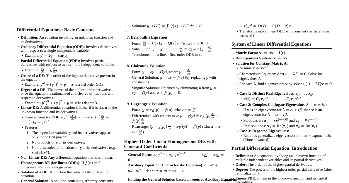
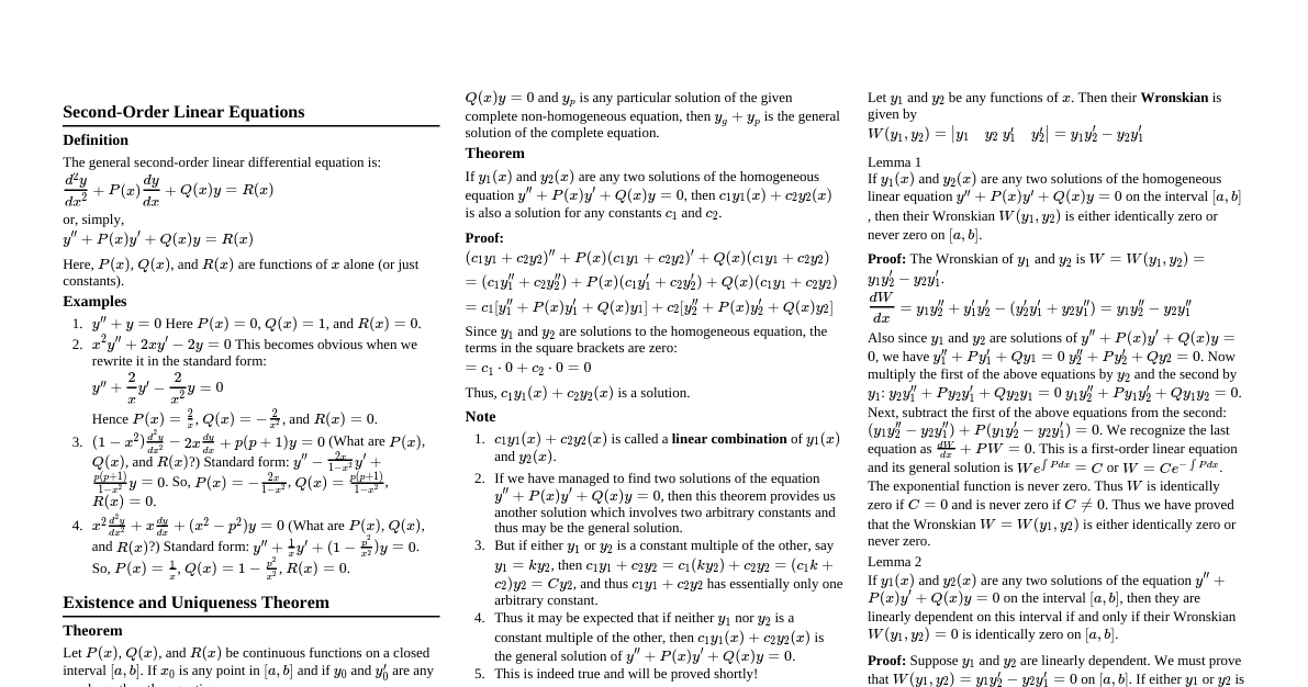
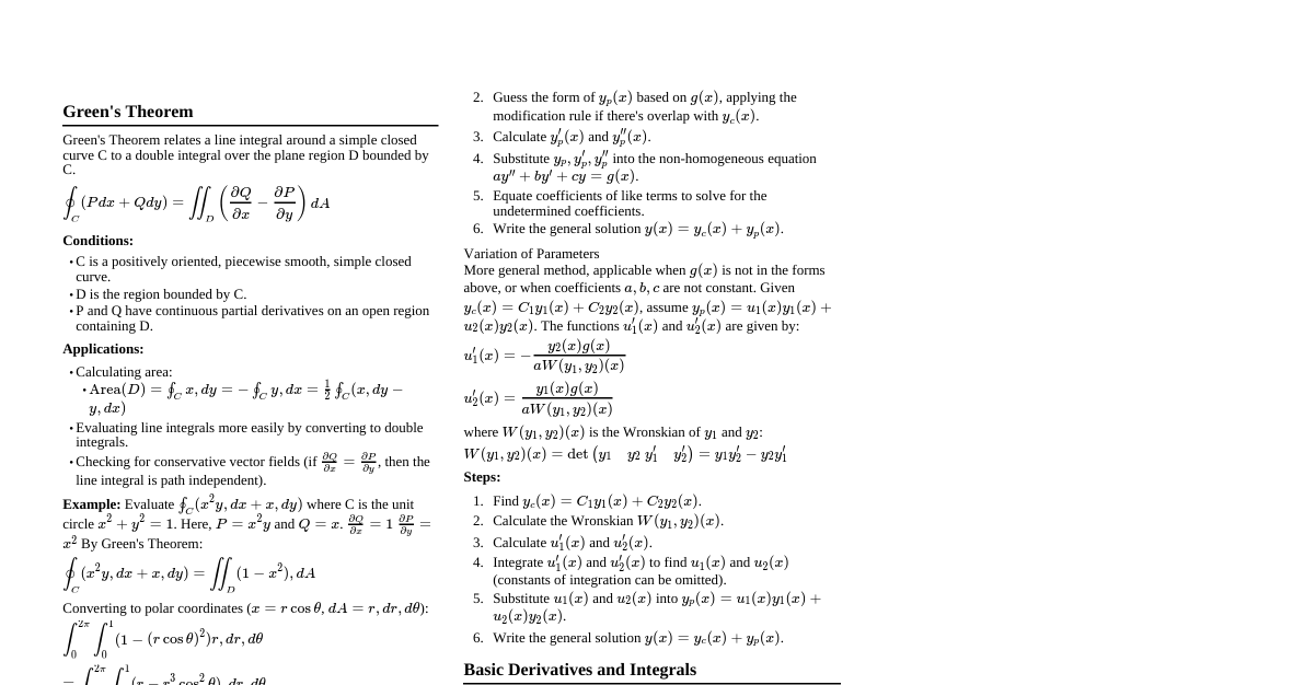
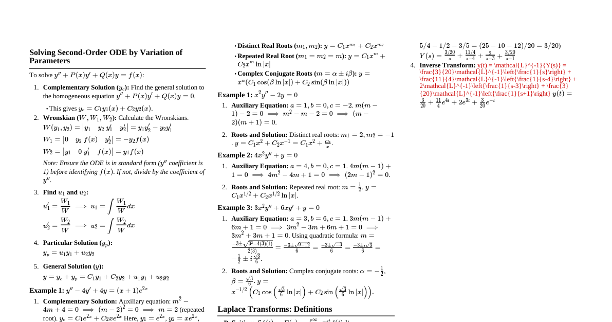
### Basics of Differential Equations A **Differential Equation** is an equation involving derivatives of an unknown function. #### Order and Degree - **Order:** The order of the highest order derivative occurring in the equation. - **Degree:** The power of the highest order derivative occurring in the equation, after making it free from radicals and fractions in its derivatives, and finding it in the form of a polynomial equation in its derivatives. - *Example:* $(d^2y/dx^2)^3 + y(dy/dx) + \sin(x) = 0$ - Order = 2 - Degree = 3 - *Example:* $d^2y/dx^2 = (x-y)\sin(x)$ - Order = 2 - Degree = 1 - **Degree Not Defined:** If the equation cannot be expressed as a polynomial in its derivatives (e.g., if derivatives are inside non-polynomial functions like $\sin(dy/dx)$). #### Formation of a Differential Equation 1. Differentiate $n$ times where $n$ is the number of arbitrary constants. 2. Eliminate the arbitrary constants to obtain the required differential equation. - *Example:* $y = A e^{mx} + B e^{-mx}$ - $y' = A m e^{mx} - B m e^{-mx}$ - $y'' = A m^2 e^{mx} + B m^2 e^{-mx} = m^2 (A e^{mx} + B e^{-mx}) = m^2 y$ - So, $y'' - m^2 y = 0$ is the differential equation. ### First-Order Differential Equations #### 1. Variable Separable Method A differential equation of the form $dy/dx = f(x, y)$ can be separated if $f(x, y) = g(x)h(y)$. Then $dy/h(y) = g(x)dx$. Integrate both sides. - *Example:* $dy/dx = (1-x)/y$ - $y dy = (1-x) dx$ - $\int y dy = \int (1-x) dx$ - $y^2/2 = x - x^2/2 + C$ #### 2. Homogeneous Differential Equation A differential equation $dy/dx = f(x, y)$ is homogeneous if $f(x, y)$ can be expressed as $f(y/x)$ or $f(x/y)$. - **Method:** Substitute $y = vx \implies dy/dx = v + x(dv/dx)$. - This transforms the equation into a variable separable form in terms of $v$ and $x$. - *Example:* $dy/dx = (x+y)/x = 1 + y/x$ - Let $y=vx$, $dy/dx = v + x(dv/dx)$ - $v + x(dv/dx) = 1 + v$ - $x(dv/dx) = 1 \implies dv = dx/x$ - $\int dv = \int dx/x \implies v = \ln|x| + C$ - Substitute back $v=y/x$: $y/x = \ln|x| + C \implies y = x(\ln|x| + C)$ #### 3. Linear Equations (First Order) A first-order linear differential equation has the form $dy/dx + P(x)y = Q(x)$, where $P(x)$ and $Q(x)$ are functions of $x$ (or constants). - **Solution:** $y \cdot IF = \int Q(x) \cdot IF dx + C$ - **Integrating Factor (IF):** $IF = e^{\int P(x)dx}$ - *Example:* $dy/dx + 2y = e^{-3x}$ - Here $P(x) = 2$, $Q(x) = e^{-3x}$ - $IF = e^{\int 2dx} = e^{2x}$ - $y \cdot e^{2x} = \int e^{-3x} \cdot e^{2x} dx + C$ - $y e^{2x} = \int e^{-x} dx + C$ - $y e^{2x} = -e^{-x} + C \implies y = -e^{-3x} + C e^{-2x}$ ### Exact Differential Equations A differential equation $M(x, y)dx + N(x, y)dy = 0$ is **exact** if $\partial M/\partial y = \partial N/\partial x$. - **Solution:** $\int M(x,y) dx$ (treating $y$ as constant) $+ \int N(x,y) dy$ (terms of N independent of x) $= C$ #### Rules for Finding Integrating Factor (IF) if Not Exact 1. **Rule 1:** If $(1/N)(\partial M/\partial y - \partial N/\partial x) = f(x)$ (a function of $x$ alone), then $IF = e^{\int f(x)dx}$. 2. **Rule 2:** If $(1/M)(\partial N/\partial x - \partial M/\partial y) = g(y)$ (a function of $y$ alone), then $IF = e^{\int g(y)dy}$. 3. **Rule 3:** If $Mdx + Ndy = 0$ is homogeneous and $Mx + Ny \ne 0$, then $IF = 1/(Mx + Ny)$. 4. **Rule 4:** If $Mdx + Ndy = 0$ is of the form $f_1(xy)y dx + f_2(xy)x dy = 0$ and $Mx - Ny \ne 0$, then $IF = 1/(Mx - Ny)$. #### Common Exact Differentials | Expression | Exact Differential | | :--------- | :----------------- | | $x dy + y dx$ | $d(xy)$ | | $(x dy - y dx) / x^2$ | $d(y/x)$ | | $(y dx - x dy) / y^2$ | $d(x/y)$ | | $(x dy - y dx) / (x^2 + y^2)$ | $d(\arctan(y/x))$ | | $(y dx - x dy) / (x^2 + y^2)$ | $d(\arctan(x/y))$ | | $(x dx + y dy) / (x^2 + y^2)$ | $1/2 d(\ln(x^2+y^2))$ | | $x dx + y dy$ | $1/2 d(x^2+y^2)$ | | $(x dy + y dx) / xy$ | $d(\ln(xy))$ | | $(x dy - y dx) / xy$ | $d(\ln(y/x))$ | ### Higher-Order Linear Differential Equations #### Linear Differential Equations with Constant Coefficients General form: $a_n y^{(n)} + a_{n-1} y^{(n-1)} + ... + a_1 y' + a_0 y = F(x)$ **1. Homogeneous Equation ($F(x) = 0$): Complementary Function (CF)** - Form the auxiliary equation (AE) by replacing $d^k y/dx^k$ with $m^k$: $a_n m^n + a_{n-1} m^{n-1} + ... + a_1 m + a_0 = 0$ - Find the roots of the AE. The form of the CF depends on the nature of these roots: - **Real and Distinct ($m_1, m_2, ...$):** $y_c = C_1 e^{m_1 x} + C_2 e^{m_2 x} + ...$ - **Real and Repeated ($m_1$ repeated $k$ times):** $y_c = (C_1 + C_2 x + ... + C_k x^{k-1})e^{m_1 x}$ - **Complex Conjugate ($a \pm ib$):** $y_c = e^{ax}(C_1 \cos(bx) + C_2 \sin(bx))$ - **Complex Conjugate Repeated ($a \pm ib$ repeated $k$ times):** $y_c = e^{ax}[(C_1 + C_2 x + ... + C_k x^{k-1})\cos(bx) + (D_1 + D_2 x + ... + D_k x^{k-1})\sin(bx)]$ **2. Non-Homogeneous Equation ($F(x) \ne 0$): Particular Integral (PI)** The general solution is $y = y_c + y_p$. The particular integral $y_p$ can be found using various methods: **Method of Undetermined Coefficients (for specific forms of $F(x)$):** | $F(x)$ | Trial $y_p$ (if no term in $F(x)$ is a solution to $y_c$) | Modification if a term in $F(x)$ is a solution to $y_c$ | | :----- | :------------------------------------------------------ | :------------------------------------------------------- | | $k e^{ax}$ | $A e^{ax}$ | $x^s A e^{ax}$ (where $s$ is multiplicity of $a$ as root of AE) | | $k \sin(ax)$ or $k \cos(ax)$ | $A \cos(ax) + B \sin(ax)$ | $x^s (A \cos(ax) + B \sin(ax))$ | | $k x^n$ (polynomial) | $A_n x^n + ... + A_1 x + A_0$ | $x^s (A_n x^n + ... + A_0)$ (where $s$ is multiplicity of $0$ as root of AE) | | $k e^{ax} \sin(bx)$ or $k e^{ax} \cos(bx)$ | $e^{ax}(A \cos(bx) + B \sin(bx))$ | $x^s e^{ax}(A \cos(bx) + B \sin(bx))$ | | $P_n(x) e^{ax}$ | $(A_n x^n + ... + A_0)e^{ax}$ | $x^s (A_n x^n + ... + A_0)e^{ax}$ | **Operator Method (using $D = d/dx$):** For $f(D)y = F(x)$, $y_p = (1/f(D))F(x)$. - **Case 1: $F(x) = e^{ax}$** - $y_p = (1/f(D))e^{ax} = (1/f(a))e^{ax}$, provided $f(a) \ne 0$. - If $f(a) = 0$, then $y_p = x \cdot (1/f'(a))e^{ax}$. If $f'(a)=0$, repeat. - **Case 2: $F(x) = \sin(ax)$ or $\cos(ax)$** - $y_p = (1/f(D^2))\sin(ax) = (1/f(-a^2))\sin(ax)$, provided $f(-a^2) \ne 0$. - If $f(-a^2) = 0$, then $y_p = x/2a \cdot (-1/f'(D^2)) \cos(ax)$ (for $\sin(ax)$) or $x/2a \cdot (1/f'(D^2)) \sin(ax)$ (for $\cos(ax)$). - **Case 3: $F(x) = x^m$ (polynomial)** - $y_p = (1/f(D))x^m$. Expand $1/f(D)$ using binomial theorem up to $D^m$. - **Case 4: $F(x) = e^{ax}V(x)$** - $y_p = (1/f(D))e^{ax}V(x) = e^{ax}(1/f(D+a))V(x)$. Then apply other rules for $V(x)$. - **Case 5: $F(x) = xV(x)$** - $y_p = (1/f(D))xV(x) = x(1/f(D))V(x) - (f'(D)/(f(D)^2))V(x)$. #### Cauchy's Equation (Euler-Cauchy Equation) Form: $a_n x^n (d^n y/dx^n) + ... + a_1 x (dy/dx) + a_0 y = F(x)$ - **Method:** 1. Substitute $x = e^z \implies z = \ln x$. 2. Let $D = d/dz$. 3. $x(dy/dx) = Dy$ 4. $x^2(d^2y/dx^2) = D(D-1)y$ 5. $x^3(d^3y/dx^3) = D(D-1)(D-2)y$, and so on. - This transforms the equation into a linear differential equation with constant coefficients in terms of $z$. #### Lagrange's Equation (Legendre's Linear Equation) Form: $a_n (ax+b)^n (d^n y/dx^n) + ... + a_1 (ax+b) (dy/dx) + a_0 y = F(x)$ - **Method:** 1. Substitute $ax+b = e^z \implies z = \ln(ax+b)$. 2. Let $D = d/dz$. 3. $(ax+b)(dy/dx) = a Dy$ 4. $(ax+b)^2(d^2y/dx^2) = a^2 D(D-1)y$, and so on. - This also transforms the equation into a linear differential equation with constant coefficients in terms of $z$. ### Family of Curves To find the differential equation of a family of curves: 1. Differentiate the given equation of the family of curves as many times as there are arbitrary constants. 2. Eliminate the arbitrary constants from the original equation and the derived equations. - *Example:* Family of circles $x^2 + y^2 = a^2$ - Differentiate: $2x + 2y (dy/dx) = 0 \implies x + y (dy/dx) = 0$ - This is the differential equation for the family of circles centered at the origin. ### Orthogonal Trajectories An **orthogonal trajectory** is a curve that intersects every curve of a given family at right angles (orthogonally). **Steps to find Orthogonal Trajectories (OT):** 1. **Given:** A family of curves $F(x, y, c) = 0$. 2. **Form the Differential Equation (DE):** Differentiate $F(x, y, c) = 0$ with respect to $x$ and eliminate the arbitrary constant $c$ to get $dy/dx = f(x, y)$. 3. **Form the DE for OT:** Replace $dy/dx$ with $-1/(dy/dx)$ (i.e. $-dx/dy$) in the DE from step 2. This gives the DE of the orthogonal trajectories: $-dx/dy = f(x, y)$ or $dy/dx = -1/f(x, y)$. 4. **Integrate:** Solve the new differential equation to find the family of orthogonal trajectories. #### Orthogonal Trajectories in Polar Coordinates 1. **Given:** A family of curves $F(r, \theta, c) = 0$. 2. **Form the DE:** Differentiate $F(r, \theta, c) = 0$ with respect to $\theta$ and eliminate $c$ to get $dr/d\theta = f(r, \theta)$. 3. **Form the DE for OT:** Replace $dr/d\theta$ with $-r^2 (d\theta/dr)$ in the DE from step 2. - So, $-r^2 (d\theta/dr) = f(r, \theta)$ or $dr/d\theta = -r^2 / f(r, \theta)$. 4. **Integrate:** Solve the new differential equation. #### Self-Orthogonal Families A family of curves is self-orthogonal if its differential equation is identical to the differential equation of its orthogonal trajectories. #### Table of Orthogonal Trajectories for Common Families | Family of Curves | Differential Equation $dy/dx = f(x, y)$ | DE of OT $dy/dx = -1/f(x, y)$ | Orthogonal Trajectory | | :--------------------------------------------- | :-------------------------------------- | :----------------------------- | :-------------------------------------- | | $y = cx$ (Lines through origin) | $y/x$ | $-x/y$ | $x^2+y^2=k^2$ (Circles centered at origin) | | $x^2+y^2=c^2$ (Circles centered at origin) | $-x/y$ | $y/x$ | $y=kx$ (Lines through origin) | | $y^2 = cx$ (Parabolas with vertex at origin, opening right) | $y/(2x)$ | $-2x/y$ | $2x^2+y^2=k$ (Ellipses centered at origin) | | $x^2+y^2=2cx$ (Circles tangent to y-axis at origin) | $(y^2-x^2)/(2xy)$ | $(x^2-y^2)/(2xy)$ | $x^2+y^2=2ky$ (Circles tangent to x-axis at origin) | ### First-Order, First-Degree, Not Solvable for y These are equations where it's difficult to express $y$ explicitly in terms of $x$ and $p = dy/dx$. #### 1. Solvable for P If the equation can be written as $P = f(x, y)$, or $y = f(x, P)$, or $x = f(y, P)$. - **Method:** Factorize the equation into linear factors of $P$. - $(P - f_1(x,y))(P - f_2(x,y))... = 0$ - Then solve each $P = f_i(x,y)$ equation as a first-order DE. - The general solution is the product of the solutions from each factor. - *Example:* $P^2 - 5P + 6 = 0 \implies (P-2)(P-3) = 0$ - $P=2 \implies dy/dx = 2 \implies y = 2x + C_1$ - $P=3 \implies dy/dx = 3 \implies y = 3x + C_2$ - General Solution: $(y-2x-C_1)(y-3x-C_2) = 0$ #### 2. Solvable for Y ($y = f(x, P)$) - **Method:** Differentiate with respect to $x$. This usually leads to a first-order linear differential equation in $x$ and $P$. Solve it for $x$ in terms of $P$. Then combine $y=f(x,P)$ and $x=g(P)$ (from the solution) to get the parametric solution in terms of $P$. - **Clairaut's Equation:** A special case where $y = Px + f(P)$. - **General Solution:** Replace $P$ with $c$: $y = cx + f(c)$. - **Singular Solution (Envelope):** Differentiate $f(P)$ with respect to $P$, set $x + f'(P) = 0$, and eliminate $P$ between this and the original equation. - *Example:* $y = Px + P^2$ - General Solution: $y = cx + c^2$ - Singular Solution: $x + 2P = 0 \implies P = -x/2$. Substitute into original: $y = (-x/2)x + (-x/2)^2 = -x^2/2 + x^2/4 = -x^2/4$. #### 3. Solvable for X ($x = f(y, P)$) - **Method:** Differentiate with respect to $y$. This usually leads to a first-order linear differential equation in $y$ and $P$. Solve it for $y$ in terms of $P$. Then combine $x=f(y,P)$ and $y=g(P)$ (from the solution) to get the parametric solution in terms of $P$. - *Example:* $x = y/P + P$ - $dx/dy = 1/P - y/P^2 (dP/dy) + dP/dy$ - Since $dx/dy = 1/P$: $1/P = 1/P - y/P^2 (dP/dy) + dP/dy$ - $0 = (-y/P^2 + 1)dP/dy$ - This gives either $dP/dy = 0 \implies P=c \implies x=y/c+c$ (general solution) - Or $-y/P^2 + 1 = 0 \implies y=P^2$. Substitute into original: $x = P^2/P + P = P+P=2P$. - So, $x=2P, y=P^2$ is the parametric singular solution. Eliminating $P$ gives $y=(x/2)^2 = x^2/4$. ### Singular Solutions A **singular solution** is a solution to a differential equation that cannot be obtained from the general solution by assigning particular values to the arbitrary constants. It often represents the envelope of the family of curves given by the general solution. #### Methods to find Singular Solutions: 1. **From General Solution:** If the general solution is $F(x, y, c) = 0$, differentiate it partially with respect to $c$ and set $\partial F/\partial c = 0$. Eliminate $c$ between $F=0$ and $\partial F/\partial c = 0$. 2. **From Differential Equation (using P):** If the differential equation is $f(x, y, P) = 0$, differentiate it partially with respect to $P$ and set $\partial f/\partial P = 0$. Eliminate $P$ between $f=0$ and $\partial f/\partial P = 0$. #### Discriminant - **P-discriminant:** From $f(x, y, P) = 0$, the P-discriminant is obtained by eliminating $P$ from $f=0$ and $\partial f/\partial P = 0$. It may contain the singular solution and/or other loci. - **C-discriminant:** From $F(x, y, c) = 0$, the C-discriminant is obtained by eliminating $c$ from $F=0$ and $\partial F/\partial c = 0$. It may contain the singular solution and/or other loci. **Loci obtained from Discriminants:** | Locus | P-discriminant | C-discriminant | | :--------------------- | :------------- | :------------- | | Envelope (Singular Sol.) | Yes | Yes | | Cusp Locus | Yes | No | | Node Locus | Yes | No | | Tac Locus | Yes | Yes | ### Wronskian For a set of $n$ functions $f_1(x), f_2(x), ..., f_n(x)$, the Wronskian $W(f_1, ..., f_n)$ is defined as the determinant: $$ W(f_1, ..., f_n)(x) = \begin{vmatrix} f_1 & f_2 & \dots & f_n \\ f_1' & f_2' & \dots & f_n' \\ \vdots & \vdots & \ddots & \vdots \\ f_1^{(n-1)} & f_2^{(n-1)} & \dots & f_n^{(n-1)} \end{vmatrix} $$ **Application:** - If $f_1, ..., f_n$ are solutions to a homogeneous linear differential equation $a_n(x)y^{(n)} + ... + a_1(x)y' + a_0(x)y = 0$, then: - The functions are **linearly independent** if and only if $W(f_1, ..., f_n)(x) \ne 0$ for at least one $x$ in the interval. - The functions are **linearly dependent** if $W(f_1, ..., f_n)(x) = 0$ for all $x$ in the interval. ### Variation of Parameters Method for finding a particular solution $y_p$ for non-homogeneous linear differential equations: $y'' + P(x)y' + Q(x)y = R(x)$ 1. Find the complementary solution $y_c = c_1 y_1(x) + c_2 y_2(x)$ for the homogeneous equation $y'' + P(x)y' + Q(x)y = 0$. 2. The particular solution is $y_p = u_1(x)y_1(x) + u_2(x)y_2(x)$, where - $u_1'(x) = -y_2(x)R(x)/W(y_1, y_2)$ - $u_2'(x) = y_1(x)R(x)/W(y_1, y_2)$ - $W(y_1, y_2) = y_1 y_2' - y_2 y_1'$ is the Wronskian of $y_1$ and $y_2$. 3. Integrate $u_1'$ and $u_2'$ to find $u_1$ and $u_2$. 4. The general solution is $y = y_c + y_p$.