Hypothesis Testing Cheatsheet
Cheatsheet Content
Hypothesis Testing: Basic Concepts Definition: Hypothesis testing is an area of statistical inference in which one evaluates a conjecture about some characteristic of the parent population based upon the information contained in the random sample. Statistical Hypothesis: A claim concerning one or more populations whose truthfulness can be established using sample data. Null vs. Alternative Hypothesis Null Hypothesis ($H_0$): A statistical hypothesis which the researcher doubts to be true. Alternative Hypothesis ($H_a$ or $H_1$): The operational statement of the theory that the researcher believes to be true and wishes to prove. Note: $H_0$ and $H_a$ are nonoverlapping statements; one and only one of the two is true. Formulating Hypotheses for Population Mean ($\mu$) Null Hypothesis Possible Alternative Hypotheses $\mu = \mu_0$ $\mu > \mu_0$ $\mu $\mu \neq \mu_0$ where $\mu_0$ is the hypothesized value. One-tailed vs. Two-tailed Tests One-tailed test: The alternative hypothesis specifies a one-directional difference for the parameter of interest. Example: $H_0: \mu_M = \mu_F$ vs. $H_a: \mu_M > \mu_F$ (males taller than females) Two-tailed test: The alternative hypothesis does not specify a directional difference for the parameter of interest. Example: $H_0: p_T = p_A$ vs. $H_a: p_T \neq p_A$ (proportions differ) Test Statistic A statistic whose value is calculated from sample measurements and on which the statistical decision will be based. Possible decisions: Reject $H_0$ Do not reject $H_0$ Critical vs. Acceptance Region Critical region (rejection region): Set of values of the test statistic for which the null hypothesis will be rejected. Acceptance region (nonrejection region): Set of values of the test statistic for which the null hypothesis will not be rejected. If the computed test statistic falls within the critical region, reject $H_0$. Otherwise, do not reject $H_0$. The acceptance and rejection regions are separated by the critical value . The location of the region of rejection depends on $H_a$. 0 1.645 (critical value) ACCEPTANCE REGION CRITICAL REGION 0 1.645 If the computed test statistic falls within this shaded region then we reject $H_0$. Otherwise, we do not reject $H_0$. Type I vs. Type II Error Type I error: Rejecting the null hypothesis when it is actually true. Type II error: Not rejecting the null hypothesis when it is actually false. DECISION NULL HYPOTHESIS True False Reject $H_0$ Type I error Correct decision Do not Reject $H_0$ Correct decision Type II error Example: $H_0$: Suspect is innocent, $H_a$: Suspect is guilty. Type I Error: Saying the suspect is guilty when they are actually innocent. Type II Error: Saying the suspect is innocent when they are actually guilty. Level of Significance ($\alpha$) The maximum probability of a Type I Error that a researcher is willing to commit. Common values: $0.01, 0.05, 0.1$. Larger $\alpha$ values lead to larger critical regions. A lower $\alpha$ implies a "stricter" test. P-value The probability of selecting a sample whose computed value for the test statistic is equal to or more extreme (in the direction stated in $H_a$) than the realized value computed from the sample data, given that the null hypothesis is true. It is the smallest level of significance at which $H_0$ will be rejected based on the information contained in the sample. Decision Rule: When p-value $\le \alpha$, reject $H_0$. Otherwise, do not reject $H_0$. Hypothesis Tests for Mean (One Population) $H_0: \mu = \mu_0$ Case Alternative Hypothesis Test Statistic Region of Rejection $\sigma$ is known $\mu $Z = \frac{\bar{X} - \mu_0}{\sigma/\sqrt{n}}$ $Z $\mu > \mu_0$ $Z > Z_\alpha$ $\mu \neq \mu_0$ $|Z| > Z_{\alpha/2}$ $\sigma$ is unknown, $n \le 30$ $\mu $T = \frac{\bar{X} - \mu_0}{s/\sqrt{n}}$ $T $\mu > \mu_0$ $T > t_{\alpha, \nu=n-1}$ $\mu \neq \mu_0$ $|T| > t_{\alpha/2, \nu=n-1}$ $\sigma$ is unknown, $n > 30$ $\mu $Z = \frac{\bar{X} - \mu_0}{s/\sqrt{n}}$ $Z $\mu > \mu_0$ $Z > Z_\alpha$ $\mu \neq \mu_0$ $|Z| > Z_{\alpha/2}$ Remarks: Formulas hold strictly for random samples from a normal distribution. The third test (unknown $\sigma$, $n > 30$) provides a good approximate test when the distribution is not normal, provided $n \ge 30$. Hypothesis Testing for Proportion (Single Population) $H_0: p = p_0$ If the unknown proportion is not expected to be too close to 0 or 1 and $n$ is large, a large sample approximation is given by: Test Statistic Alternative Hypothesis Region of Rejection $Z = \frac{Y - np_0}{\sqrt{np_0(1 - p_0)}}$ $p $Z $p > p_0$ $Z > Z_\alpha$ $p \neq p_0$ $|Z| > Z_{\alpha/2}$ where $Y$ is the number of "successes" in the sample. Hypothesis Tests for Difference of Means (Two Populations) For Independent Sampling, $H_0: \mu_X - \mu_Y = d_0$ Let $(X_1, ..., X_{n_1})$ be a random sample with mean $\mu_X$ and variance $\sigma_X^2$. Let $(Y_1, ..., Y_{n_2})$ be a random sample with mean $\mu_Y$ and variance $\sigma_Y^2$. Let $\bar{X}$ and $\bar{Y}$ denote the sample mean and $S_X^2$ and $S_Y^2$ denote the sample variance of the two random samples, respectively. Case 1: $\sigma_X^2$ and $\sigma_Y^2$ are known Alternative Hypothesis Test Statistic Region of Rejection $\mu_X - \mu_Y $Z = \frac{(\bar{X} - \bar{Y}) - d_0}{\sqrt{\frac{\sigma_X^2}{n_1} + \frac{\sigma_Y^2}{n_2}}}$ $Z $\mu_X - \mu_Y > d_0$ $Z > Z_\alpha$ $\mu_X - \mu_Y \neq d_0$ $|Z| > Z_{\alpha/2}$ Case 2: $\sigma_X^2$ and $\sigma_Y^2$ are unknown but $\sigma_X^2 = \sigma_Y^2$ Alternative Hypothesis Test Statistic Region of Rejection $\mu_X - \mu_Y $T = \frac{(\bar{X} - \bar{Y}) - d_0}{S_p \sqrt{\frac{1}{n_1} + \frac{1}{n_2}}}$ $S_p = \sqrt{\frac{(n_1-1)S_X^2 + (n_2-1)S_Y^2}{n_1+n_2-2}}$ $T $\mu_X - \mu_Y > d_0$ $T > t_{\alpha, \nu=n_1+n_2-2}$ $\mu_X - \mu_Y \neq d_0$ $|T| > t_{\alpha/2, \nu=n_1+n_2-2}$ Case 3: $\sigma_X^2$ and $\sigma_Y^2$ are unknown but $\sigma_X^2 \neq \sigma_Y^2$ Alternative Hypothesis Test Statistic Region of Rejection $\mu_X - \mu_Y $T = \frac{(\bar{X} - \bar{Y}) - d_0}{\sqrt{\frac{S_X^2}{n_1} + \frac{S_Y^2}{n_2}}}$ $v = \frac{\left(\frac{S_X^2}{n_1} + \frac{S_Y^2}{n_2}\right)^2}{\frac{(S_X^2/n_1)^2}{n_1-1} + \frac{(S_Y^2/n_2)^2}{n_2-1}}$ $T $\mu_X - \mu_Y > d_0$ $T > t_{\alpha, \nu}$ $\mu_X - \mu_Y \neq d_0$ $|T| > t_{\alpha/2, \nu}$ Case 4: $\sigma_X^2$ and $\sigma_Y^2$ are unknown, $n_1$ and $n_2 > 30$ Alternative Hypothesis Test Statistic Region of Rejection $\mu_X - \mu_Y $Z = \frac{(\bar{X} - \bar{Y}) - d_0}{\sqrt{\frac{S_X^2}{n_1} + \frac{S_Y^2}{n_2}}}$ $Z $\mu_X - \mu_Y > d_0$ $Z > Z_\alpha$ $\mu_X - \mu_Y \neq d_0$ $|Z| > Z_{\alpha/2}$ Flowchart for Independent Sampling ($\mu_X - \mu_Y$) $\sigma_X^2$ and $\sigma_Y^2$ known? Use case 1 $n_1 > 30$ $n_2 > 30$? Use case 4 $n_1 = n_2$? Use case 2 $\sigma_X^2 = \sigma_Y^2$? Use case 3 Yes No Yes No Yes No No For Paired Sampling, $H_0: \mu_D = \mu_X - \mu_Y = d_0$ Let $\{(X_1, Y_1), (X_2, Y_2), ..., (X_n, Y_n)\}$ be your sample data. Denote $D_i = X_i - Y_i$ for $i=1, 2, ..., n$. $\bar{D} = \frac{1}{n} \sum_{i=1}^n D_i = \bar{X} - \bar{Y}$ $S_D = \sqrt{\frac{\sum_{i=1}^n (D_i - \bar{D})^2}{n-1}}$ Test Statistic Alternative Hypothesis Region of Rejection $T = \frac{\bar{D} - d_0}{S_D/\sqrt{n}}$ $\mu_X - \mu_Y $T $\mu_X - \mu_Y > d_0$ $T > t_{\alpha, \nu=n-1}$ $\mu_X - \mu_Y \neq d_0$ $|T| > t_{\alpha/2, \nu=n-1}$ Hypothesis Tests for Difference of Proportions (Two Populations) $H_0: p_X - p_Y = d_0$ Assuming independent samples of size $n_1$ and $n_2$ from two binomial populations, the sample proportions $\hat{p}_X$ and $\hat{p}_Y$ are computed as follows: Test Statistic Alternative Hypothesis Region of Rejection $Z = \frac{(\hat{p}_X - \hat{p}_Y) - d_0}{\sqrt{\hat{p}(1-\hat{p})\left(\frac{1}{n_1} + \frac{1}{n_2}\right)}}$ where $\hat{p} = \frac{X+Y}{n_1+n_2}$ $p_X - p_Y $Z $p_X - p_Y > d_0$ $Z > Z_\alpha$ $p_X - p_Y \neq d_0$ $|Z| > Z_{\alpha/2}$ where $X$ = number of elements in the 1st sample possessing the characteristic of interest and $Y$ = number of elements in the 2nd sample possessing the characteristic of interest. We require the sample sizes $n_1 \ge 30$ and $n_2 \ge 30$ (or the sample sizes are large). Chi-square Distribution and Test for Independence Test for Independence The chi-square ($\chi^2$) test for independence is used to determine whether two categorical variables are related or not. Observations are tallied in an $r \times c$ contingency table. EDUCATIONAL ATTAINMENT NUMBER OF CHILDREN TOTAL 0-1 2-3 Over 3 Elementary 14 37 32 83 Secondary 19 42 17 78 College 12 17 10 39 TOTAL 45 96 59 200 Hypotheses for Test for Independence $H_0$: The two variables are independent. $H_a$: The two variables are not independent. Test Statistic for Independence $\chi^2 = \sum_{i=1}^r \sum_{j=1}^c \frac{(O_{ij} - E_{ij})^2}{E_{ij}}$ where: $O_{ij}$ = observed number of cases in the $i$-th row of the $j$-th column $E_{ij}$ = expected number of cases under $H_0$ $E_{ij} = \frac{\text{(i-th row total)(j-th column total)}}{\text{grand total}}$ Decision Rule: Reject $H_0$ if $\chi^2 > \chi^2_{\alpha, (r-1)(c-1)}$. Remarks on Test for Independence The test is valid if at least 80% of the cells have expected frequencies of at least 5 and no cell has an expected frequency $\le 1$. If many expected frequencies are very small, researchers commonly combine categories of variables to obtain a table having larger cell frequencies. Yates' Correction for Continuity (for 2x2 contingency tables) For a 2x2 contingency table, a correction called Yates' correction for continuity is applied. The test statistic then becomes: $\chi^2 = \sum_{i=1}^r \sum_{j=1}^c \frac{(|O_{ij} - E_{ij}| - 0.5)^2}{E_{ij}}$ This formula may be used if the number of observations $\ge 40$. It may still be used if the number of observations is between 20 and 40 provided that all expected frequencies are $> 5$. If the above conditions are not met for the 2x2 case then alternatives may be used.