Laplace & Fourier Transforms

Cheatsheet Content

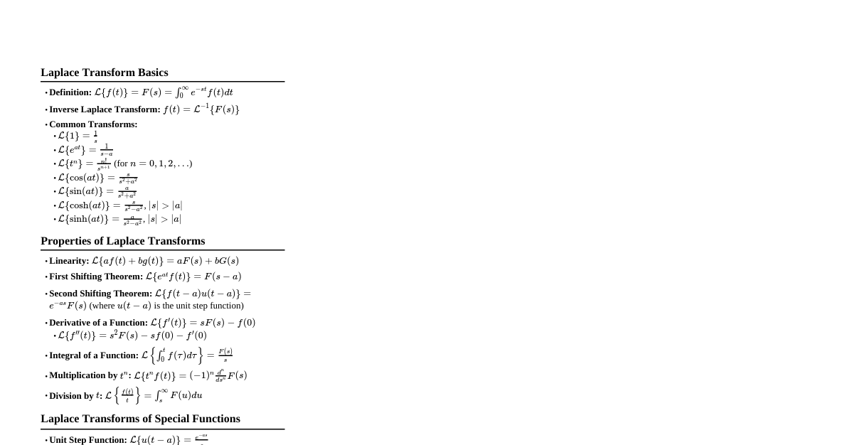
Laplace Transform The Laplace Transform is a powerful tool for solving linear differential equations with constant coefficients, especially those with initial conditions. It transforms a function of time $f(t)$ into a function of a complex frequency variable $s$. Definition For a function $f(t)$ defined for $t \ge 0$, its Laplace Transform $\mathcal{L}\{f(t)\}$ is given by: $$F(s) = \mathcal{L}\{f(t)\} = \int_0^\infty e^{-st} f(t) dt$$ where $s = \sigma + j\omega$ is a complex variable. The integral converges for $\text{Re}(s) > \alpha$, where $\alpha$ is the abscissa of convergence. Inverse Laplace Transform The inverse Laplace Transform $\mathcal{L}^{-1}\{F(s)\}$ recovers the original time-domain function: $$f(t) = \mathcal{L}^{-1}\{F(s)\} = \frac{1}{2\pi j} \int_{\sigma-j\infty}^{\sigma+j\infty} e^{st} F(s) ds$$ This is a complex contour integral, typically solved using tables or residue theorem. Properties of Laplace Transform Linearity: $\mathcal{L}\{af(t) + bg(t)\} = aF(s) + bG(s)$ Time Shifting: $\mathcal{L}\{f(t-a)u(t-a)\} = e^{-as}F(s)$ for $a \ge 0$ Example: $\mathcal{L}\{e^{-2(t-3)}u(t-3)\} = e^{-3s}\mathcal{L}\{e^{-2t}u(t)\} = e^{-3s}\frac{1}{s+2}$ Frequency Shifting: $\mathcal{L}\{e^{at}f(t)\} = F(s-a)$ Example: $\mathcal{L}\{e^{3t}\cos(2t)u(t)\}$. Here $f(t)=\cos(2t)u(t)$, so $F(s) = \frac{s}{s^2+2^2}$. Applying frequency shifting with $a=3$, we get $\frac{s-3}{(s-3)^2+4}$. Time Differentiation: $\mathcal{L}\{f'(t)\} = sF(s) - f(0)$ $\mathcal{L}\{f''(t)\} = s^2F(s) - sf(0) - f'(0)$ Example: Solve $y'(t) + 2y(t) = e^{-t}$ with $y(0)=1$. Taking Laplace Transform of both sides: $$[sY(s) - y(0)] + 2Y(s) = \frac{1}{s+1}$$ $$sY(s) - 1 + 2Y(s) = \frac{1}{s+1}$$ $$(s+2)Y(s) = 1 + \frac{1}{s+1} = \frac{s+2}{s+1}$$ $$Y(s) = \frac{1}{s+1}$$ Taking inverse Laplace Transform: $y(t) = e^{-t}u(t)$. Time Integration: $\mathcal{L}\left\{\int_0^t f(\tau) d\tau\right\} = \frac{1}{s}F(s)$ Example: $\mathcal{L}\left\{\int_0^t \sin(\tau) d\tau\right\} = \frac{1}{s} \mathcal{L}\{\sin(t)\} = \frac{1}{s} \frac{1}{s^2+1} = \frac{1}{s(s^2+1)}$ Frequency Differentiation: $\mathcal{L}\{tf(t)\} = -\frac{d}{ds}F(s)$ Example: $\mathcal{L}\{t\sin(t)\}$. Here $f(t)=\sin(t)$, so $F(s)=\frac{1}{s^2+1}$. $$\mathcal{L}\{t\sin(t)\} = -\frac{d}{ds}\left(\frac{1}{s^2+1}\right) = - \frac{-(2s)}{(s^2+1)^2} = \frac{2s}{(s^2+1)^2}$$ Convolution: $\mathcal{L}\{(f*g)(t)\} = F(s)G(s)$ Example: Find the output $y(t)$ of an LTI system with impulse response $h(t)=e^{-t}u(t)$ and input $x(t)=u(t)$. We know $y(t) = (h*x)(t)$. $H(s) = \mathcal{L}\{e^{-t}u(t)\} = \frac{1}{s+1}$ $X(s) = \mathcal{L}\{u(t)\} = \frac{1}{s}$ $Y(s) = H(s)X(s) = \frac{1}{s(s+1)}$ Using partial fraction expansion: $Y(s) = \frac{1}{s} - \frac{1}{s+1}$. Inverse Laplace Transform: $y(t) = (u(t) - e^{-t}u(t)) = (1-e^{-t})u(t)$. Common Laplace Transform Pairs $f(t)$ $F(s) = \mathcal{L}\{f(t)\}$ Region of Convergence $\delta(t)$ (Dirac Delta) $1$ All $s$ $u(t)$ (Unit Step) $\frac{1}{s}$ $\text{Re}(s) > 0$ $t^n u(t)$ $\frac{n!}{s^{n+1}}$ $\text{Re}(s) > 0$ $e^{at}u(t)$ $\frac{1}{s-a}$ $\text{Re}(s) > \text{Re}(a)$ $\sin(\omega t)u(t)$ $\frac{\omega}{s^2+\omega^2}$ $\text{Re}(s) > 0$ $\cos(\omega t)u(t)$ $\frac{s}{s^2+\omega^2}$ $\text{Re}(s) > 0$ $e^{at}\sin(\omega t)u(t)$ $\frac{\omega}{(s-a)^2+\omega^2}$ $\text{Re}(s) > \text{Re}(a)$ $e^{at}\cos(\omega t)u(t)$ $\frac{s-a}{(s-a)^2+\omega^2}$ $\text{Re}(s) > \text{Re}(a)$ $t e^{at}u(t)$ $\frac{1}{(s-a)^2}$ $\text{Re}(s) > \text{Re}(a)$ Fourier Transform The Fourier Transform decomposes a function (signal) into its constituent frequencies. It is particularly useful for analyzing signals in the frequency domain and solving partial differential equations. Continuous-Time Fourier Transform (CTFT) For a function $f(t)$ integrable over $(-\infty, \infty)$, its CTFT $\mathcal{F}\{f(t)\}$ is given by: $$F(\omega) = \mathcal{F}\{f(t)\} = \int_{-\infty}^\infty f(t) e^{-j\omega t} dt$$ where $\omega$ is the angular frequency (in rad/s). Inverse Continuous-Time Fourier Transform (ICTFT) The inverse CTFT $\mathcal{F}^{-1}\{F(\omega)\}$ recovers the original time-domain function: $$f(t) = \mathcal{F}^{-1}\{F(\omega)\} = \frac{1}{2\pi} \int_{-\infty}^\infty F(\omega) e^{j\omega t} d\omega$$ Properties of Fourier Transform Linearity: $\mathcal{F}\{af(t) + bg(t)\} = aF(\omega) + bG(\omega)$ Time Shifting: $\mathcal{F}\{f(t-t_0)\} = e^{-j\omega t_0}F(\omega)$ Example: If $\mathcal{F}\{\text{rect}(t)\} = \text{sinc}(\omega/2)$, then $\mathcal{F}\{\text{rect}(t-1)\} = e^{-j\omega} \text{sinc}(\omega/2)$. Frequency Shifting: $\mathcal{F}\{e^{j\omega_0 t}f(t)\} = F(\omega-\omega_0)$ Example: $\mathcal{F}\{\cos(\omega_0 t)\} = \mathcal{F}\left\{\frac{e^{j\omega_0 t} + e^{-j\omega_0 t}}{2}\right\} = \frac{1}{2}\mathcal{F}\{e^{j\omega_0 t}\} + \frac{1}{2}\mathcal{F}\{e^{-j\omega_0 t}\}$. Using frequency shifting with $f(t)=1$ (whose FT is $2\pi\delta(\omega)$): $\mathcal{F}\{e^{j\omega_0 t}\} = 2\pi\delta(\omega-\omega_0)$ $\mathcal{F}\{e^{-j\omega_0 t}\} = 2\pi\delta(\omega+\omega_0)$ So, $\mathcal{F}\{\cos(\omega_0 t)\} = \pi[\delta(\omega-\omega_0) + \delta(\omega+\omega_0)]$. Time Scaling: $\mathcal{F}\{f(at)\} = \frac{1}{|a|}F\left(\frac{\omega}{a}\right)$ Example: If $\mathcal{F}\{e^{-|t|}\} = \frac{2}{1+\omega^2}$, then $\mathcal{F}\{e^{-2|t|}\} = \frac{1}{2}\frac{2}{1+(\omega/2)^2} = \frac{1}{1+\omega^2/4} = \frac{4}{4+\omega^2}$. Time Differentiation: $\mathcal{F}\left\{\frac{d^n f(t)}{dt^n}\right\} = (j\omega)^n F(\omega)$ Example: Let $f(t) = e^{-at}u(t)$, then $F(\omega) = \frac{1}{a+j\omega}$. $\mathcal{F}\{f'(t)\} = \mathcal{F}\{-ae^{-at}u(t) + \delta(t)\} = -a\frac{1}{a+j\omega} + 1 = \frac{-a + a+j\omega}{a+j\omega} = \frac{j\omega}{a+j\omega}$. From the property: $\mathcal{F}\{f'(t)\} = j\omega F(\omega) = j\omega \frac{1}{a+j\omega}$. This matches. Convolution: $\mathcal{F}\{(f*g)(t)\} = F(\omega)G(\omega)$ Example: Find the output $y(t)$ of an LTI system with input $x(t)=e^{-t}u(t)$ and impulse response $h(t)=e^{-2t}u(t)$. $X(\omega) = \frac{1}{1+j\omega}$ $H(\omega) = \frac{1}{2+j\omega}$ $Y(\omega) = X(\omega)H(\omega) = \frac{1}{(1+j\omega)(2+j\omega)}$ Using partial fraction expansion: $Y(\omega) = \frac{1}{1+j\omega} - \frac{1}{2+j\omega}$. Inverse Fourier Transform: $y(t) = e^{-t}u(t) - e^{-2t}u(t) = (e^{-t}-e^{-2t})u(t)$. Parseval's Theorem: $\int_{-\infty}^\infty |f(t)|^2 dt = \frac{1}{2\pi} \int_{-\infty}^\infty |F(\omega)|^2 d\omega$ Example: For $f(t)=e^{-at}u(t)$ ($a>0$), $\int_0^\infty (e^{-at})^2 dt = \int_0^\infty e^{-2at} dt = \left[-\frac{1}{2a}e^{-2at}\right]_0^\infty = \frac{1}{2a}$. $F(\omega) = \frac{1}{a+j\omega}$, so $|F(\omega)|^2 = \frac{1}{a^2+\omega^2}$. $\frac{1}{2\pi} \int_{-\infty}^\infty \frac{1}{a^2+\omega^2} d\omega = \frac{1}{2\pi} \left[\frac{1}{a}\arctan\left(\frac{\omega}{a}\right)\right]_{-\infty}^\infty = \frac{1}{2\pi a} \left(\frac{\pi}{2} - (-\frac{\pi}{2})\right) = \frac{1}{2\pi a}(\pi) = \frac{1}{2a}$. This matches. Common Fourier Transform Pairs $f(t)$ $F(\omega) = \mathcal{F}\{f(t)\}$ $\delta(t)$ $1$ $1$ $2\pi\delta(\omega)$ $u(t)$ $\pi\delta(\omega) + \frac{1}{j\omega}$ $e^{-at}u(t)$ ($a>0$) $\frac{1}{a+j\omega}$ $e^{at}u(-t)$ ($a>0$) $\frac{1}{a-j\omega}$ $e^{-a|t|}$ ($a>0$) $\frac{2a}{a^2+\omega^2}$ $\text{rect}\left(\frac{t}{\tau}\right)$ (Pulse) $\tau \text{sinc}\left(\frac{\omega\tau}{2}\right) = \tau \frac{\sin(\omega\tau/2)}{\omega\tau/2}$ $\sin(\omega_0 t)$ $j\pi[\delta(\omega+\omega_0) - \delta(\omega-\omega_0)]$ $\cos(\omega_0 t)$ $\pi[\delta(\omega+\omega_0) + \delta(\omega-\omega_0)]$ $e^{j\omega_0 t}$ $2\pi\delta(\omega-\omega_0)$ Relationship Between Laplace and Fourier Transforms The Fourier Transform can be seen as a special case of the Laplace Transform. If the Region of Convergence (ROC) of $F(s)$ includes the $j\omega$-axis (i.e., $\text{Re}(s)=0$), then the Fourier Transform is obtained by setting $s=j\omega$ in the Laplace Transform: $$F(\omega) = F(s)|_{s=j\omega} = \mathcal{L}\{f(t)\}|_{s=j\omega}$$ This is only valid if $f(t)$ is absolutely integrable, i.e., $\int_{-\infty}^\infty |f(t)| dt Applications Laplace Transform Applications Solving linear ODEs with initial conditions: As shown in the Time Differentiation example, Laplace transforms convert differential equations into algebraic equations in the $s$-domain, which are easier to solve. System analysis in control theory: Transfer functions, $H(s) = Y(s)/X(s)$, are derived using Laplace transforms to analyze system stability, frequency response, and transient behavior. Circuit analysis: Capacitors and inductors are represented by impedances $1/(sC)$ and $sL$ respectively, simplifying circuit analysis in the $s$-domain. Fourier Transform Applications Signal processing (spectral analysis): Analyze the frequency content of signals (e.g., audio, seismic data) to identify dominant frequencies or noise. For example, using FFT to find the pitch of a sound. Filter design: Design filters (low-pass, high-pass) in the frequency domain to remove unwanted frequency components from a signal. Solving PDEs: Transform PDEs into algebraic equations, solve them in the frequency domain, and then inverse transform to get the solution in the original domain. For example, solving the heat equation. Image processing: Used for image compression (e.g., JPEG), noise reduction, and edge detection by manipulating frequency components of an image. Discrete Transforms (Brief Overview) Discrete-Time Fourier Transform (DTFT) For a discrete-time sequence $x[n]$: $$X(e^{j\omega}) = \sum_{n=-\infty}^\infty x[n] e^{-j\omega n}$$ The DTFT is always periodic with period $2\pi$. Discrete Fourier Transform (DFT) For a finite-length sequence $x[n]$ of length $N$ ($0 \le n \le N-1$): $$X[k] = \sum_{n=0}^{N-1} x[n] e^{-j\frac{2\pi}{N}kn}, \quad 0 \le k \le N-1$$ The DFT is a sampled version of the DTFT and is extensively used in digital signal processing, often computed efficiently using the Fast Fourier Transform (FFT) algorithm. Z-Transform The discrete-time counterpart to the Laplace Transform for discrete signals $x[n]$: $$X(z) = \sum_{n=-\infty}^\infty x[n] z^{-n}$$ where $z$ is a complex variable. The DTFT is obtained by evaluating the Z-Transform on the unit circle, $z = e^{j\omega}$, if the ROC includes the unit circle.