Linear Algebra 1 Essentials
Cheatsheet Content
1. Vectors Definition and Basic Operations Definition: A vector in $\mathbb{R}^n$ is an ordered $n$-tuple of real numbers. $\vec{v} = (v_1, v_2, \dots, v_n)$. Vector Addition: $\vec{u} + \vec{v} = (u_1+v_1, \dots, u_n+v_n)$. Example 1: $(1, 2) + (3, 4) = (4, 6)$ Example 2: $(-1, 0, 5) + (2, -3, 1) = (1, -3, 6)$ Example 3: $(0, 0) + (x, y) = (x, y)$ (Zero vector) Example 4: $(7, -2) + (-7, 2) = (0, 0)$ (Additive inverse) Example 5: $(1, 2, 3) + (4, 5, 6) = (5, 7, 9)$ Scalar Multiplication: $c\vec{v} = (cv_1, \dots, cv_n)$. Example 1: $3(1, 2) = (3, 6)$ Example 2: $-1(4, -2, 0) = (-4, 2, 0)$ Example 3: $0(5, -1) = (0, 0)$ Example 4: $2(1, 0, -3) = (2, 0, -6)$ Example 5: $\frac{1}{2}(6, 8) = (3, 4)$ Dot Product (Scalar Product) Definition: $\vec{u} \cdot \vec{v} = u_1v_1 + u_2v_2 + \dots + u_nv_n$. The result is a scalar. Properties: $\vec{u} \cdot \vec{v} = \vec{v} \cdot \vec{u}$, $\vec{u} \cdot (\vec{v} + \vec{w}) = \vec{u} \cdot \vec{v} + \vec{u} \cdot \vec{w}$. Geometric Interpretation: $\vec{u} \cdot \vec{v} = ||\vec{u}|| \cdot ||\vec{v}|| \cos \theta$. Orthogonality: $\vec{u} \perp \vec{v}$ if $\vec{u} \cdot \vec{v} = 0$. Example 1: $(1, 2) \cdot (3, 4) = 1(3) + 2(4) = 3 + 8 = 11$ Example 2: $(1, -1, 0) \cdot (1, 1, 5) = 1(1) + (-1)(1) + 0(5) = 1 - 1 + 0 = 0$ (Orthogonal) Example 3: $(2, 0, -3) \cdot (1, 1, 1) = 2(1) + 0(1) + (-3)(1) = 2 + 0 - 3 = -1$ Example 4: If $\vec{u} = (1, 0)$ and $\vec{v} = (0, 1)$, $\vec{u} \cdot \vec{v} = 0$. Example 5: $(5, 1) \cdot (2, 3) = 5(2) + 1(3) = 10 + 3 = 13$ Magnitude (Length) of a Vector Definition: $||\vec{v}|| = \sqrt{\vec{v} \cdot \vec{v}} = \sqrt{v_1^2 + v_2^2 + \dots + v_n^2}$. Unit Vector: A vector with magnitude 1. $\hat{u} = \frac{\vec{u}}{||\vec{u}||}$. Example 1: $||(3, 4)|| = \sqrt{3^2 + 4^2} = \sqrt{9 + 16} = \sqrt{25} = 5$ Example 2: $||(1, -2, 2)|| = \sqrt{1^2 + (-2)^2 + 2^2} = \sqrt{1 + 4 + 4} = \sqrt{9} = 3$ Example 3: Unit vector for $(3, 4)$ is $(\frac{3}{5}, \frac{4}{5})$. Example 4: $||(0, 0, 0)|| = 0$. Example 5: $||(2, -1)|| = \sqrt{2^2 + (-1)^2} = \sqrt{4 + 1} = \sqrt{5}$ 2. Matrices Definition and Basic Operations Definition: An $m \times n$ matrix is a rectangular array of numbers with $m$ rows and $n$ columns. Matrix Addition/Subtraction: Element-wise operation for matrices of the same size. Example 1: $\begin{pmatrix} 1 & 2 \\ 3 & 4 \end{pmatrix} + \begin{pmatrix} 5 & 6 \\ 7 & 8 \end{pmatrix} = \begin{pmatrix} 6 & 8 \\ 10 & 12 \end{pmatrix}$ Example 2: $\begin{pmatrix} 0 & 1 \\ -1 & 0 \end{pmatrix} - \begin{pmatrix} 1 & 0 \\ 0 & 1 \end{pmatrix} = \begin{pmatrix} -1 & 1 \\ -1 & -1 \end{pmatrix}$ Example 3: $\begin{pmatrix} 1 & 2 \end{pmatrix} + \begin{pmatrix} 3 & 4 \end{pmatrix} = \begin{pmatrix} 4 & 6 \end{pmatrix}$ Example 4: $\begin{pmatrix} 1 & 1 \\ 1 & 1 \end{pmatrix} + \begin{pmatrix} 0 & 0 \\ 0 & 0 \end{pmatrix} = \begin{pmatrix} 1 & 1 \\ 1 & 1 \end{pmatrix}$ Example 5: $\begin{pmatrix} 5 & 2 \\ 1 & 3 \end{pmatrix} + \begin{pmatrix} -5 & -2 \\ -1 & -3 \end{pmatrix} = \begin{pmatrix} 0 & 0 \\ 0 & 0 \end{pmatrix}$ Scalar Multiplication: Multiply each element by the scalar. Example 1: $2 \begin{pmatrix} 1 & 2 \\ 3 & 4 \end{pmatrix} = \begin{pmatrix} 2 & 4 \\ 6 & 8 \end{pmatrix}$ Example 2: $-1 \begin{pmatrix} 1 & 0 \\ 0 & 1 \end{pmatrix} = \begin{pmatrix} -1 & 0 \\ 0 & -1 \end{pmatrix}$ Example 3: $0 \begin{pmatrix} 1 & 2 \\ 3 & 4 \end{pmatrix} = \begin{pmatrix} 0 & 0 \\ 0 & 0 \end{pmatrix}$ Example 4: $\frac{1}{2} \begin{pmatrix} 4 & 6 \\ 2 & 8 \end{pmatrix} = \begin{pmatrix} 2 & 3 \\ 1 & 4 \end{pmatrix}$ Example 5: $3 \begin{pmatrix} 1 & 2 & 3 \end{pmatrix} = \begin{pmatrix} 3 & 6 & 9 \end{pmatrix}$ Matrix Multiplication Definition: If $A$ is $m \times n$ and $B$ is $n \times p$, then $AB$ is $m \times p$. $(AB)_{ij} = \sum_{k=1}^n A_{ik}B_{kj}$. (Row-column dot product). Not commutative ($AB \ne BA$). Example 1: $\begin{pmatrix} 1 & 2 \\ 3 & 4 \end{pmatrix} \begin{pmatrix} 5 & 6 \\ 7 & 8 \end{pmatrix} = \begin{pmatrix} 1(5)+2(7) & 1(6)+2(8) \\ 3(5)+4(7) & 3(6)+4(8) \end{pmatrix} = \begin{pmatrix} 19 & 22 \\ 43 & 50 \end{pmatrix}$ Example 2: $\begin{pmatrix} 1 & 0 \\ 0 & 1 \end{pmatrix} \begin{pmatrix} a & b \\ c & d \end{pmatrix} = \begin{pmatrix} a & b \\ c & d \end{pmatrix}$ (Identity matrix) Example 3: $\begin{pmatrix} 1 & 2 \end{pmatrix} \begin{pmatrix} 3 \\ 4 \end{pmatrix} = (1(3)+2(4)) = (11)$ Example 4: $\begin{pmatrix} 1 \\ 2 \end{pmatrix} \begin{pmatrix} 3 & 4 \end{pmatrix} = \begin{pmatrix} 1(3) & 1(4) \\ 2(3) & 2(4) \\ \end{pmatrix} = \begin{pmatrix} 3 & 4 \\ 6 & 8 \end{pmatrix}$ Example 5: $\begin{pmatrix} 0 & 1 \\ 0 & 0 \end{pmatrix} \begin{pmatrix} 0 & 1 \\ 0 & 0 \end{pmatrix} = \begin{pmatrix} 0 & 0 \\ 0 & 0 \end{pmatrix}$ Transpose of a Matrix Definition: $A^T$. Rows become columns and columns become rows. $(A^T)_{ij} = A_{ji}$. Properties: $(A^T)^T = A$, $(A+B)^T = A^T + B^T$, $(cA)^T = cA^T$, $(AB)^T = B^T A^T$. Example 1: If $A = \begin{pmatrix} 1 & 2 \\ 3 & 4 \end{pmatrix}$, then $A^T = \begin{pmatrix} 1 & 3 \\ 2 & 4 \end{pmatrix}$ Example 2: If $B = \begin{pmatrix} 1 & 2 & 3 \\ 4 & 5 & 6 \end{pmatrix}$, then $B^T = \begin{pmatrix} 1 & 4 \\ 2 & 5 \\ 3 & 6 \end{pmatrix}$ Example 3: If $C = \begin{pmatrix} 1 & 0 & 0 \\ 0 & 1 & 0 \\ 0 & 0 & 1 \end{pmatrix}$, then $C^T = C$ (Symmetric matrix) Example 4: If $\vec{v} = \begin{pmatrix} 1 \\ 2 \\ 3 \end{pmatrix}$, then $\vec{v}^T = \begin{pmatrix} 1 & 2 & 3 \end{pmatrix}$ Example 5: If $D = \begin{pmatrix} 2 & -1 \\ -1 & 3 \end{pmatrix}$, then $D^T = D$ 3. Systems of Linear Equations Representations Standard Form: $a_{11}x_1 + \dots + a_{1n}x_n = b_1$ $\dots$ $a_{m1}x_1 + \dots + a_{mn}x_n = b_m$ Matrix Form: $A\vec{x} = \vec{b}$, where $A$ is the coefficient matrix, $\vec{x}$ is the variable vector, and $\vec{b}$ is the constant vector. Augmented Matrix: $[A | \vec{b}]$. Example 1: $2x + 3y = 7$, $x - y = 1$ can be written as $\begin{pmatrix} 2 & 3 \\ 1 & -1 \end{pmatrix} \begin{pmatrix} x \\ y \end{pmatrix} = \begin{pmatrix} 7 \\ 1 \end{pmatrix}$ Example 2: Augmented matrix for above: $\begin{pmatrix} 2 & 3 & | & 7 \\ 1 & -1 & | & 1 \end{pmatrix}$ Example 3: $x_1 + x_2 - x_3 = 0$, $2x_1 + x_3 = 5$ is $\begin{pmatrix} 1 & 1 & -1 \\ 2 & 0 & 1 \end{pmatrix} \begin{pmatrix} x_1 \\ x_2 \\ x_3 \end{pmatrix} = \begin{pmatrix} 0 \\ 5 \end{pmatrix}$ Example 4: Augmented matrix for above: $\begin{pmatrix} 1 & 1 & -1 & | & 0 \\ 2 & 0 & 1 & | & 5 \end{pmatrix}$ Example 5: A single equation $3x - 2y = 4$ is $\begin{pmatrix} 3 & -2 \end{pmatrix} \begin{pmatrix} x \\ y \end{pmatrix} = \begin{pmatrix} 4 \end{pmatrix}$ Gaussian Elimination / Row Echelon Form (REF) Elementary Row Operations: Swap two rows. Multiply a row by a non-zero scalar. Add a multiple of one row to another row. Row Echelon Form (REF) properties: All non-zero rows are above any zero rows. The leading entry (pivot) of each non-zero row is in a column to the right of the leading entry of the row above it. All entries in a column below a leading entry are zeros. Example 1 (REF): $\begin{pmatrix} 1 & 2 & 3 \\ 0 & 1 & 4 \\ 0 & 0 & 1 \end{pmatrix}$ Example 2 (REF): $\begin{pmatrix} 1 & 2 & 3 & | & 9 \\ 0 & 1 & 4 & | & 5 \\ 0 & 0 & 0 & | & 0 \end{pmatrix}$ (Infinitely many solutions) Example 3 (REF): $\begin{pmatrix} 1 & 2 & 3 & | & 9 \\ 0 & 1 & 4 & | & 5 \\ 0 & 0 & 0 & | & 1 \end{pmatrix}$ (No solution) Example 4 (REF): $\begin{pmatrix} 1 & 0 & 0 & | & 2 \\ 0 & 1 & 0 & | & 3 \\ 0 & 0 & 1 & | & 4 \end{pmatrix}$ (Unique solution) Example 5 (REF): $\begin{pmatrix} 1 & 2 & 0 & 1 \\ 0 & 0 & 1 & 3 \\ 0 & 0 & 0 & 0 \end{pmatrix}$ Reduced Row Echelon Form (RREF) RREF properties (in addition to REF): The leading entry in each non-zero row is 1 (called a leading 1). Each column containing a leading 1 has zeros everywhere else. Example 1 (RREF): $\begin{pmatrix} 1 & 0 & 0 & | & 2 \\ 0 & 1 & 0 & | & 3 \\ 0 & 0 & 1 & | & 4 \end{pmatrix}$ (Unique solution $x=2, y=3, z=4$) Example 2 (RREF): $\begin{pmatrix} 1 & 0 & 5 & | & 7 \\ 0 & 1 & -2 & | & 3 \\ 0 & 0 & 0 & | & 0 \end{pmatrix}$ (Infinitely many solutions, $z$ is a free variable) Example 3 (RREF): $\begin{pmatrix} 1 & 0 & | & 0 \\ 0 & 1 & | & 0 \\ 0 & 0 & | & 1 \end{pmatrix}$ (No solution) Example 4 (RREF): $\begin{pmatrix} 1 & 0 & 0 \\ 0 & 1 & 0 \\ 0 & 0 & 1 \end{pmatrix}$ (Identity matrix) Example 5 (RREF): $\begin{pmatrix} 1 & 0 & -1 \\ 0 & 1 & 2 \end{pmatrix}$ 4. Inverse Matrices Definition and Properties Definition: For a square matrix $A$, if there exists a matrix $A^{-1}$ such that $AA^{-1} = A^{-1}A = I$ (Identity Matrix), then $A^{-1}$ is the inverse of $A$. Singular Matrix: A matrix that does not have an inverse. Properties: $(A^{-1})^{-1} = A$, $(AB)^{-1} = B^{-1}A^{-1}$, $(A^T)^{-1} = (A^{-1})^T$. Example 1: If $A = \begin{pmatrix} 2 & 5 \\ 1 & 3 \end{pmatrix}$, then $A^{-1} = \begin{pmatrix} 3 & -5 \\ -1 & 2 \end{pmatrix}$ (since $ADJ(A) = \begin{pmatrix} 3 & -5 \\ -1 & 2 \end{pmatrix}$ and $\det(A) = 6-5=1$) Example 2: $\begin{pmatrix} 1 & 0 \\ 0 & 1 \end{pmatrix}^{-1} = \begin{pmatrix} 1 & 0 \\ 0 & 1 \end{pmatrix}$ Example 3: $\begin{pmatrix} 1 & 2 \\ 2 & 4 \end{pmatrix}$ is singular because $\det(A) = 1(4) - 2(2) = 0$. Example 4: If $A = \begin{pmatrix} 1 & 1 \\ 0 & 1 \end{pmatrix}$, then $A^{-1} = \begin{pmatrix} 1 & -1 \\ 0 & 1 \end{pmatrix}$ Example 5: If $A = \begin{pmatrix} a & 0 \\ 0 & b \end{pmatrix}$ with $a,b \ne 0$, then $A^{-1} = \begin{pmatrix} 1/a & 0 \\ 0 & 1/b \end{pmatrix}$ Finding the Inverse using Gaussian Elimination Augment $A$ with the identity matrix: $[A | I]$. Perform row operations to transform $[A | I]$ into $[I | A^{-1}]$. Example 1: Find $A^{-1}$ for $A = \begin{pmatrix} 1 & 2 \\ 3 & 7 \end{pmatrix}$ $\begin{pmatrix} 1 & 2 & | & 1 & 0 \\ 3 & 7 & | & 0 & 1 \end{pmatrix} \xrightarrow{R_2 - 3R_1} \begin{pmatrix} 1 & 2 & | & 1 & 0 \\ 0 & 1 & | & -3 & 1 \end{pmatrix} \xrightarrow{R_1 - 2R_2} \begin{pmatrix} 1 & 0 & | & 7 & -2 \\ 0 & 1 & | & -3 & 1 \end{pmatrix}$ So, $A^{-1} = \begin{pmatrix} 7 & -2 \\ -3 & 1 \end{pmatrix}$ Example 2: Find $A^{-1}$ for $A = \begin{pmatrix} 1 & 0 & 0 \\ 0 & 2 & 0 \\ 0 & 0 & 3 \end{pmatrix}$ $\begin{pmatrix} 1 & 0 & 0 & | & 1 & 0 & 0 \\ 0 & 2 & 0 & | & 0 & 1 & 0 \\ 0 & 0 & 3 & | & 0 & 0 & 1 \end{pmatrix} \xrightarrow{\frac{1}{2}R_2, \frac{1}{3}R_3} \begin{pmatrix} 1 & 0 & 0 & | & 1 & 0 & 0 \\ 0 & 1 & 0 & | & 0 & 1/2 & 0 \\ 0 & 0 & 1 & | & 0 & 0 & 1/3 \end{pmatrix}$ So, $A^{-1} = \begin{pmatrix} 1 & 0 & 0 \\ 0 & 1/2 & 0 \\ 0 & 0 & 1/3 \end{pmatrix}$ Example 3: Find inverse of $\begin{pmatrix} 1 & 1 \\ 0 & 1 \end{pmatrix}$. Result is $\begin{pmatrix} 1 & -1 \\ 0 & 1 \end{pmatrix}$. Example 4: Try to find inverse of $\begin{pmatrix} 1 & 2 \\ 1 & 2 \end{pmatrix}$. It will lead to a row of zeros on the left side, indicating no inverse. Example 5: For $A = \begin{pmatrix} 1 & 1 & 0 \\ 0 & 1 & 1 \\ 0 & 0 & 1 \end{pmatrix}$, $A^{-1} = \begin{pmatrix} 1 & -1 & 1 \\ 0 & 1 & -1 \\ 0 & 0 & 1 \end{pmatrix}$. 5. Determinants Definition for $2 \times 2$ and $3 \times 3$ Matrices $2 \times 2$ Matrix: For $A = \begin{pmatrix} a & b \\ c & d \end{pmatrix}$, $\det(A) = ad - bc$. $3 \times 3$ Matrix (Sarrus' Rule / Cofactor Expansion): For $A = \begin{pmatrix} a & b & c \\ d & e & f \\ g & h & i \end{pmatrix}$, $\det(A) = a(ei-fh) - b(di-fg) + c(dh-eg)$. Example 1 ($2 \times 2$): $\det \begin{pmatrix} 1 & 2 \\ 3 & 4 \end{pmatrix} = 1(4) - 2(3) = 4 - 6 = -2$ Example 2 ($2 \times 2$): $\det \begin{pmatrix} 5 & -1 \\ 2 & 0 \end{pmatrix} = 5(0) - (-1)(2) = 0 + 2 = 2$ Example 3 ($3 \times 3$): $\det \begin{pmatrix} 1 & 2 & 3 \\ 0 & 1 & 4 \\ 5 & 6 & 0 \end{pmatrix} = 1(0-24) - 2(0-20) + 3(0-5) = -24 + 40 - 15 = 1$ Example 4 ($3 \times 3$): $\det \begin{pmatrix} 2 & 0 & 0 \\ 0 & 3 & 0 \\ 0 & 0 & 4 \end{pmatrix} = 2(3 \cdot 4 - 0 \cdot 0) - 0 + 0 = 2(12) = 24$ (Diagonal matrix) Example 5 ($3 \times 3$): $\det \begin{pmatrix} 1 & 2 & 3 \\ 1 & 2 & 3 \\ 4 & 5 & 6 \end{pmatrix} = 0$ (Two identical rows) Properties of Determinants $\det(A^T) = \det(A)$. $\det(AB) = \det(A)\det(B)$. $\det(A^{-1}) = 1/\det(A)$ (if $A$ is invertible). If a matrix has a row/column of zeros, $\det(A) = 0$. If a matrix has two identical rows/columns, $\det(A) = 0$. If a matrix is triangular (upper or lower), its determinant is the product of its diagonal entries. Example 1: If $\det(A) = 2$ and $\det(B) = 3$, then $\det(AB) = 2 \cdot 3 = 6$. Example 2: If $A = \begin{pmatrix} 1 & 2 \\ 0 & 3 \end{pmatrix}$, $\det(A) = 1 \cdot 3 = 3$. Example 3: $\det \begin{pmatrix} 1 & 2 \\ 0 & 0 \end{pmatrix} = 0$. Example 4: $\det \begin{pmatrix} 1 & 2 \\ 1 & 2 \end{pmatrix} = 0$. Example 5: If $\det(A) = 5$, then $\det(A^{-1}) = 1/5$. Cramer's Rule Used to solve systems of linear equations using determinants. For $A\vec{x} = \vec{b}$, $x_j = \frac{\det(A_j)}{\det(A)}$, where $A_j$ is the matrix formed by replacing the $j$-th column of $A$ with $\vec{b}$. Example 1: Solve $2x + y = 7$, $x + 3y = 11$. $A = \begin{pmatrix} 2 & 1 \\ 1 & 3 \end{pmatrix}$, $\det(A) = 5$. $A_1 = \begin{pmatrix} 7 & 1 \\ 11 & 3 \end{pmatrix}$, $\det(A_1) = 21 - 11 = 10$. $A_2 = \begin{pmatrix} 2 & 7 \\ 1 & 11 \end{pmatrix}$, $\det(A_2) = 22 - 7 = 15$. $x = \frac{10}{5} = 2$, $y = \frac{15}{5} = 3$. Example 2: Solve $x - y = 1$, $x + y = 5$. $A = \begin{pmatrix} 1 & -1 \\ 1 & 1 \end{pmatrix}$, $\det(A) = 2$. $A_1 = \begin{pmatrix} 1 & -1 \\ 5 & 1 \end{A_1} \end{pmatrix}$, $\det(A_1) = 6$. $A_2 = \begin{pmatrix} 1 & 1 \\ 1 & 5 \end{A_2} \end{pmatrix}$, $\det(A_2) = 4$. $x = 3$, $y = 2$. Example 3: For $3x + 2y = 1$, $x + y = 0$. $x=1, y=-1$. Example 4: For $x + y = 2$, $x = 1$. $A_1 = \begin{pmatrix} 2 & 1 \\ 1 & 0 \end{pmatrix}, A_2 = \begin{pmatrix} 1 & 2 \\ 1 & 1 \end{pmatrix}$ Example 5: For $2x+y=0, x-y=3$. $x=1, y=-2$. 6. Vector Spaces and Subspaces Vector Space Definition A non-empty set $V$ of objects, called vectors, on which two operations are defined: vector addition and scalar multiplication, satisfying ten axioms. Axioms (examples): Closure under addition ($\vec{u}+\vec{v} \in V$), associative addition, commutative addition, zero vector, additive inverse, closure under scalar multiplication ($c\vec{u} \in V$), distributive properties. Example 1: $\mathbb{R}^n$ with standard addition and scalar multiplication is a vector space. Example 2: The set of all $m \times n$ matrices, $M_{m \times n}$, forms a vector space. Example 3: The set of all polynomials of degree at most $n$, $P_n$, is a vector space. Example 4: The set of all continuous real-valued functions on an interval $[a, b]$, $C[a,b]$, is a vector space. Example 5: The set of all solutions to a homogeneous linear differential equation is a vector space. Subspaces A subset $W$ of a vector space $V$ is a subspace if: The zero vector of $V$ is in $W$. $W$ is closed under vector addition (if $\vec{u}, \vec{v} \in W$, then $\vec{u}+\vec{v} \in W$). $W$ is closed under scalar multiplication (if $\vec{u} \in W$ and $c$ is a scalar, then $c\vec{u} \in W$). Example 1: The set of all vectors of the form $(a, b, 0)$ is a subspace of $\mathbb{R}^3$. Example 2: The set of all $2 \times 2$ symmetric matrices is a subspace of $M_{2 \times 2}$. Example 3: The set of all polynomials $p(x)$ in $P_n$ such that $p(0) = 0$ is a subspace. Example 4: The set $\{(x, y) | y = 2x\}$ is a subspace of $\mathbb{R}^2$. Example 5: The set of all solutions to a homogeneous system $A\vec{x} = \vec{0}$ (Null Space/Kernel) is a subspace. Span of a Set of Vectors The span of a set of vectors $\{\vec{v}_1, \dots, \vec{v}_k\}$ is the set of all possible linear combinations of these vectors: $\text{span}\{\vec{v}_1, \dots, \vec{v}_k\} = \{c_1\vec{v}_1 + \dots + c_k\vec{v}_k \mid c_i \in \mathbb{R}\}$. The span is always a subspace. Example 1: The span of $\{(1, 0)\}$ in $\mathbb{R}^2$ is the x-axis. Example 2: The span of $\{(1, 0), (0, 1)\}$ in $\mathbb{R}^2$ is all of $\mathbb{R}^2$. Example 3: The span of $\{(1, 1), (2, 2)\}$ is the line $y=x$. Example 4: The span of $\{(1, 0, 0), (0, 1, 0)\}$ in $\mathbb{R}^3$ is the xy-plane. Example 5: Is $(3, 5)$ in the span of $\{(1, 2), (1, 1)\}$? Yes, $2(1,2) + 1(1,1) = (3,5)$. 7. Linear Independence and Basis Linear Independence A set of vectors $\{\vec{v}_1, \dots, \vec{v}_k\}$ is linearly independent if the only solution to the vector equation $c_1\vec{v}_1 + \dots + c_k\vec{v}_k = \vec{0}$ is $c_1 = \dots = c_k = 0$. If there are non-zero solutions for $c_i$, the vectors are linearly dependent. Example 1: $\{(1, 0), (0, 1)\}$ in $\mathbb{R}^2$ is linearly independent. ($c_1(1,0) + c_2(0,1) = (0,0) \implies c_1=0, c_2=0$) Example 2: $\{(1, 1), (2, 2)\}$ in $\mathbb{R}^2$ is linearly dependent. ($2(1,1) - 1(2,2) = (0,0)$) Example 3: $\{(1, 0, 0), (0, 1, 0), (0, 0, 1)\}$ in $\mathbb{R}^3$ is linearly independent. Example 4: $\{(1, 2), (3, 4), (5, 6)\}$ in $\mathbb{R}^2$ is linearly dependent (more vectors than dimension). Example 5: The columns of an invertible matrix are linearly independent. Basis of a Vector Space A set of vectors $B = \{\vec{v}_1, \dots, \vec{v}_n\}$ is a basis for a vector space $V$ if: $B$ is linearly independent. $B$ spans $V$. Standard Basis: The set of unit vectors $\vec{e}_1, \dots, \vec{e}_n$. Example 1: The standard basis for $\mathbb{R}^2$ is $\{(1, 0), (0, 1)\}$. Example 2: The standard basis for $P_2$ (polynomials of degree $\le 2$) is $\{1, x, x^2\}$. Example 3: $\{(1, 1), (1, -1)\}$ is a basis for $\mathbb{R}^2$. Example 4: For $M_{2 \times 2}$, a basis is $\left\{ \begin{pmatrix} 1 & 0 \\ 0 & 0 \end{pmatrix}, \begin{pmatrix} 0 & 1 \\ 0 & 0 \end{pmatrix}, \begin{pmatrix} 0 & 0 \\ 1 & 0 \end{pmatrix}, \begin{pmatrix} 0 & 0 \\ 0 & 1 \end{pmatrix} \right\}$. Example 5: Any set of $n$ linearly independent vectors in $\mathbb{R}^n$ forms a basis for $\mathbb{R}^n$. Dimension of a Vector Space The dimension of a vector space $V$, denoted $\text{dim}(V)$, is the number of vectors in any basis for $V$. Example 1: $\text{dim}(\mathbb{R}^n) = n$. So, $\text{dim}(\mathbb{R}^3) = 3$. Example 2: $\text{dim}(P_n) = n+1$. So, $\text{dim}(P_2) = 3$. Example 3: $\text{dim}(M_{m \times n}) = mn$. So, $\text{dim}(M_{2 \times 2}) = 4$. Example 4: The dimension of the subspace $\{(x, y, 0) | x, y \in \mathbb{R}\}$ in $\mathbb{R}^3$ is 2. Example 5: The dimension of the zero vector space $\{\vec{0}\}$ is 0. 8. Rank and Nullity Column Space (Image) and Row Space Column Space ($\text{Col}(A)$): The span of the column vectors of $A$. It is a subspace of $\mathbb{R}^m$ for an $m \times n$ matrix $A$. Row Space ($\text{Row}(A)$): The span of the row vectors of $A$. It is a subspace of $\mathbb{R}^n$ for an $m \times n$ matrix $A$. Rank: $\text{rank}(A) = \text{dim}(\text{Col}(A)) = \text{dim}(\text{Row}(A))$. This is the number of pivot positions in the RREF of $A$. Example 1: For $A = \begin{pmatrix} 1 & 2 \\ 2 & 4 \end{pmatrix}$, $\text{Col}(A) = \text{span}\left\{ \begin{pmatrix} 1 \\ 2 \end{pmatrix} \right\}$. $\text{rank}(A) = 1$. Example 2: For $A = \begin{pmatrix} 1 & 0 & 0 \\ 0 & 1 & 0 \\ 0 & 0 & 1 \end{pmatrix}$, $\text{Col}(A) = \mathbb{R}^3$. $\text{rank}(A) = 3$. Example 3: Basis for $\text{Col}(A)$ are the pivot columns of $A$. For $A = \begin{pmatrix} 1 & 2 & 0 \\ 0 & 0 & 1 \end{pmatrix}$, basis is $\left\{ \begin{pmatrix} 1 \\ 0 \end{pmatrix}, \begin{pmatrix} 0 \\ 1 \end{pmatrix} \right\}$. $\text{rank}(A) = 2$. Example 4: Basis for $\text{Row}(A)$ are the non-zero rows of the RREF of $A$. For $A = \begin{pmatrix} 1 & 2 & 3 \\ 1 & 2 & 3 \end{pmatrix}$, RREF is $\begin{pmatrix} 1 & 2 & 3 \\ 0 & 0 & 0 \end{pmatrix}$. Basis for $\text{Row}(A)$ is $\{(1, 2, 3)\}$. $\text{rank}(A) = 1$. Example 5: If $A$ is an $n \times n$ invertible matrix, $\text{rank}(A) = n$. Null Space (Kernel) Null Space ($\text{Nul}(A)$ or $\text{Ker}(A)$): The set of all solutions to the homogeneous equation $A\vec{x} = \vec{0}$. It is a subspace of $\mathbb{R}^n$ for an $m \times n$ matrix $A$. Nullity: $\text{nullity}(A) = \text{dim}(\text{Nul}(A))$. This is the number of free variables in the solution to $A\vec{x} = \vec{0}$. Rank-Nullity Theorem: For an $m \times n$ matrix $A$, $\text{rank}(A) + \text{nullity}(A) = n$. Example 1: For $A = \begin{pmatrix} 1 & 2 \\ 2 & 4 \end{pmatrix}$, $A\vec{x} = \vec{0} \implies x_1 + 2x_2 = 0 \implies x_1 = -2x_2$. Basis for $\text{Nul}(A)$ is $\left\{ \begin{pmatrix} -2 \\ 1 \end{pmatrix} \right\}$. $\text{nullity}(A) = 1$. Example 2: For $A = \begin{pmatrix} 1 & 0 & 0 \\ 0 & 1 & 0 \\ 0 & 0 & 1 \end{pmatrix}$, $A\vec{x} = \vec{0} \implies \vec{x} = \vec{0}$. Basis for $\text{Nul}(A)$ is $\{\}$. $\text{nullity}(A) = 0$. Example 3: For $A = \begin{pmatrix} 1 & 2 & 3 \\ 0 & 0 & 0 \end{pmatrix}$, $x_1 + 2x_2 + 3x_3 = 0$. $x_2, x_3$ are free variables. $\vec{x} = x_2 \begin{pmatrix} -2 \\ 1 \\ 0 \end{pmatrix} + x_3 \begin{pmatrix} -3 \\ 0 \\ 1 \end{pmatrix}$. Basis for $\text{Nul}(A)$ is $\left\{ \begin{pmatrix} -2 \\ 1 \\ 0 \end{pmatrix}, \begin{pmatrix} -3 \\ 0 \\ 1 \end{pmatrix} \right\}$. $\text{nullity}(A) = 2$. Example 4: Using Rank-Nullity for previous example: $n=3$, $\text{rank}(A)=1$, so $1 + \text{nullity}(A) = 3 \implies \text{nullity}(A) = 2$. Example 5: If $\text{Nul}(A) = \{\vec{0}\}$, then $\text{rank}(A) = n$. This means columns are linearly independent. 9. Eigenvalues and Eigenvectors Definitions Eigenvector: A non-zero vector $\vec{x}$ such that for a square matrix $A$, $A\vec{x} = \lambda\vec{x}$ for some scalar $\lambda$. Eigenvalue: The scalar $\lambda$ associated with an eigenvector $\vec{x}$. Characteristic Equation: $\det(A - \lambda I) = 0$. The roots of this polynomial are the eigenvalues. Example 1: For $A = \begin{pmatrix} 2 & 0 \\ 0 & 3 \end{pmatrix}$, $\begin{pmatrix} 2 & 0 \\ 0 & 3 \end{pmatrix} \begin{pmatrix} 1 \\ 0 \end{pmatrix} = \begin{pmatrix} 2 \\ 0 \end{pmatrix} = 2 \begin{pmatrix} 1 \\ 0 \end{pmatrix}$. So $\lambda=2$ is an eigenvalue, $\begin{pmatrix} 1 \\ 0 \end{pmatrix}$ is an eigenvector. Example 2: For the same $A$, $\begin{pmatrix} 2 & 0 \\ 0 & 3 \end{pmatrix} \begin{pmatrix} 0 \\ 1 \end{pmatrix} = \begin{pmatrix} 0 \\ 3 \end{pmatrix} = 3 \begin{pmatrix} 0 \\ 1 \end{pmatrix}$. So $\lambda=3$ is an eigenvalue, $\begin{pmatrix} 0 \\ 1 \end{pmatrix}$ is an eigenvector. Example 3: Find eigenvalues for $A = \begin{pmatrix} 2 & 1 \\ 1 & 2 \end{pmatrix}$. $\det \begin{pmatrix} 2-\lambda & 1 \\ 1 & 2-\lambda \end{pmatrix} = (2-\lambda)^2 - 1 = 0 \implies (2-\lambda)^2 = 1 \implies 2-\lambda = \pm 1$. $\lambda_1 = 1$, $\lambda_2 = 3$. Example 4: Find eigenvectors for $\lambda=1$ from Example 3: $(A - 1I)\vec{x} = \begin{pmatrix} 1 & 1 \\ 1 & 1 \end{pmatrix} \begin{pmatrix} x_1 \\ x_2 \end{pmatrix} = \begin{pmatrix} 0 \\ 0 \end{pmatrix} \implies x_1 + x_2 = 0 \implies x_1 = -x_2$. Eigenvector: $\begin{pmatrix} -1 \\ 1 \end{pmatrix}$ (or any scalar multiple). Example 5: Find eigenvectors for $\lambda=3$ from Example 3: $(A - 3I)\vec{x} = \begin{pmatrix} -1 & 1 \\ 1 & -1 \end{pmatrix} \begin{pmatrix} x_1 \\ x_2 \end{pmatrix} = \begin{pmatrix} 0 \\ 0 \end{pmatrix} \implies -x_1 + x_2 = 0 \implies x_1 = x_2$. Eigenvector: $\begin{pmatrix} 1 \\ 1 \end{pmatrix}$ (or any scalar multiple). Eigenspace For a given eigenvalue $\lambda$, the set of all eigenvectors corresponding to $\lambda$, together with the zero vector, forms a subspace called the eigenspace $E_\lambda$. $E_\lambda = \text{Nul}(A - \lambda I)$. Example 1: For $A = \begin{pmatrix} 2 & 1 \\ 1 & 2 \end{pmatrix}$, the eigenspace for $\lambda=1$ is $\text{span}\left\{ \begin{pmatrix} -1 \\ 1 \end{pmatrix} \right\}$. Example 2: The eigenspace for $\lambda=3$ is $\text{span}\left\{ \begin{pmatrix} 1 \\ 1 \end{pmatrix} \right\}$. Example 3: For an identity matrix $I = \begin{pmatrix} 1 & 0 \\ 0 & 1 \end{pmatrix}$, $\lambda=1$ is an eigenvalue. $E_1 = \text{Nul}(I - 1I) = \text{Nul}(\begin{pmatrix} 0 & 0 \\ 0 & 0 \end{pmatrix}) = \mathbb{R}^2$. Example 4: For $A = \begin{pmatrix} 0 & 1 \\ 0 & 0 \end{pmatrix}$, $\lambda=0$ is the only eigenvalue. $E_0 = \text{Nul}\begin{pmatrix} 0 & 1 \\ 0 & 0 \end{pmatrix} = \text{span}\left\{ \begin{pmatrix} 1 \\ 0 \end{pmatrix} \right\}$. Example 5: The dimension of an eigenspace is called the geometric multiplicity of the eigenvalue.