Complex Analysis & PDE
Cheatsheet Content
Complex Variable Functions Analytic Functions Let $f(z) = u + iv$ be a complex function. $f(z)$ is analytic if: $u_x, u_y, v_x, v_y$ are continuous. It satisfies the Cauchy-Riemann (C-R) equations: $u_x = v_y$ $u_y = -v_x$ C-R Equations (Polar Form): $u_r = \frac{1}{r} v_\theta$ $v_r = -\frac{1}{r} u_\theta$ Harmonic Functions A function $u(x,y)$ is harmonic if it satisfies Laplace's equation: $\nabla^2 u = u_{xx} + u_{yy} = 0$. If $f(z) = u + iv$ is analytic, then $u$ and $v$ are harmonic functions. To check if $u,v$ are harmonic: Find $u_x, u_y, v_x, v_y$. Check if $u_{xx} + u_{yy} = 0$ and $v_{xx} + v_{yy} = 0$. If both are zero, they are harmonic. Finding Conjugate Harmonic Function $v$ from $u$ Given $u(x,y)$, to find $v(x,y)$: Use C-R equation $v_y = u_x$. Integrate $u_x$ with respect to $y$ to get $v(x,y) = \int u_x dy + \phi(x)$. Differentiate $v(x,y)$ with respect to $x$: $v_x = \frac{\partial}{\partial x} (\int u_x dy) + \phi'(x)$. Use the other C-R equation $v_x = -u_y$. Equate the two expressions for $v_x$ to find $\phi'(x)$. Integrate $\phi'(x)$ with respect to $x$ to find $\phi(x)$. (If $\phi'(x)=0$, then $\phi(x)=C$). Substitute $\phi(x)$ back into the expression for $v(x,y)$. Then write $f(z) = u(x,y) + i v(x,y)$. Cauchy Integral Theorem & Formulas Cauchy Integral Theorem If $f(z)$ is analytic inside and on a simple closed contour $C$, then $\oint_C f(z) dz = 0$. Note: Pole $z=a$ of order $n$ means $(z-a)^n$ is in the denominator. Cauchy Integral Formula If $f(z)$ is analytic inside and on a simple closed contour $C$, and $a$ is any point inside $C$: $$ f(a) = \frac{1}{2\pi i} \oint_C \frac{f(z)}{z-a} dz $$ For derivatives: $$ f^{(n)}(a) = \frac{n!}{2\pi i} \oint_C \frac{f(z)}{(z-a)^{n+1}} dz $$ Residue Theorem Residue at a simple pole ($z=z_0$): $$ \text{Res}_{z=z_0} f(z) = \lim_{z \to z_0} (z-z_0) f(z) $$ Residue at a pole of order $m$ ($z=z_0$): $$ \text{Res}_{z=z_0} f(z) = \frac{1}{(m-1)!} \lim_{z \to z_0} \frac{d^{m-1}}{dz^{m-1}} [(z-z_0)^m f(z)] $$ Cauchy Residue Theorem: If $f(z)$ is analytic inside and on a simple closed contour $C$, except for a finite number of isolated singularities $z_1, z_2, \dots, z_n$ inside $C$, then: $$ \oint_C f(z) dz = 2\pi i \sum_{k=1}^n \text{Res}_{z=z_k} f(z) $$ Partial Differential Equations (PDE) Formation of PDEs By eliminating arbitrary constants: Given an equation $F(x,y,z,a,b)=0$. Differentiate with respect to $x$ to get $p = \frac{\partial z}{\partial x}$. Differentiate with respect to $y$ to get $q = \frac{\partial z}{\partial y}$. Eliminate constants $a, b$ from the original equation and the two partial derivatives. By eliminating arbitrary functions: Given an equation $F(u,v)=0$ where $u$ and $v$ are functions of $x,y,z$. Differentiate $F(u,v)=0$ with respect to $x$ and $y$. Eliminate the function $F$ from the resulting equations. Solving PDEs Direct Integration Integrate with respect to the variable indicated by the partial derivative, treating other variables as constants. Remember to add an arbitrary function of the "constant" variable(s) instead of a constant. Example: If $\frac{\partial^2 z}{\partial x \partial y} = f(x,y)$, integrate with respect to $y$ first, then $x$. Lagrange's Method for Linear First-Order PDEs For PDEs of the form $Pp + Qq = R$ (where $P, Q, R$ are functions of $x,y,z$): Write the auxiliary equations: $\frac{dx}{P} = \frac{dy}{Q} = \frac{dz}{R}$. Solve these ordinary differential equations to find two independent solutions, $u(x,y,z) = a$ and $v(x,y,z) = b$. The general solution is given by $\Phi(u,v) = 0$ or $u = \phi(v)$. Method of Separation of Variables Assume the solution $u(x,t)$ can be written as a product of functions of single variables, e.g., $u(x,t) = X(x)T(t)$. Substitute this into the PDE. Separate the variables such that one side depends only on $x$ and the other only on $t$. Equate both sides to a constant (separation constant, e.g., $\lambda$). Solve the resulting two ordinary differential equations for $X(x)$ and $T(t)$. Combine $X(x)$ and $T(t)$ to get the general solution. Use initial and boundary conditions to find the constants. Applications of Separation of Variables 1D Wave Equation: $\frac{\partial^2 u}{\partial t^2} = c^2 \frac{\partial^2 u}{\partial x^2}$ Solution form: $u(x,t) = (C_1 \cos(kx) + C_2 \sin(kx))(C_3 \cos(ckt) + C_4 \sin(ckt))$ 1D Heat Equation: $\frac{\partial u}{\partial t} = c^2 \frac{\partial^2 u}{\partial x^2}$ Solution form: $u(x,t) = e^{-c^2 k^2 t} (C_1 \cos(kx) + C_2 \sin(kx))$ Fourier Transform Integral Transform of a Function General form: $F(s) = \int_{x_1}^{x_2} f(x) K(s,x) dx$ Laplace Transform Kernel: $K(s,x) = e^{-sx}$ Fourier Transform Kernel: $K(s,x) = e^{isx}$ Fourier Integral Representation For a function $f(x)$ defined on $(-\infty, \infty)$: $$ f(x) = \frac{1}{\pi} \int_0^\infty \int_{-\infty}^\infty f(t) \cos(\lambda(t-x)) dt d\lambda $$ Alternatively: $$ f(x) = \int_0^\infty [A(\lambda) \cos(\lambda x) + B(\lambda) \sin(\lambda x)] d\lambda $$ where $A(\lambda) = \frac{1}{\pi} \int_{-\infty}^\infty f(t) \cos(\lambda t) dt$ and $B(\lambda) = \frac{1}{\pi} \int_{-\infty}^\infty f(t) \sin(\lambda t) dt$. Fourier Sine and Cosine Integral If $f(x)$ is an even function: $$ f(x) = \int_0^\infty A(\lambda) \cos(\lambda x) d\lambda $$ where $A(\lambda) = \frac{2}{\pi} \int_0^\infty f(t) \cos(\lambda t) dt$. If $f(x)$ is an odd function: $$ f(x) = \int_0^\infty B(\lambda) \sin(\lambda x) d\lambda $$ where $B(\lambda) = \frac{2}{\pi} \int_0^\infty f(t) \sin(\lambda t) dt$. Fourier Transform (FT) Full Fourier Transform: $\mathcal{F}\{f(x)\} = F(s) = \int_{-\infty}^\infty f(x) e^{isx} dx$ Fourier Sine Transform: $\mathcal{F}_s\{f(x)\} = F_s(s) = \int_0^\infty f(x) \sin(sx) dx$ Fourier Cosine Transform: $\mathcal{F}_c\{f(x)\} = F_c(s) = \int_0^\infty f(x) \cos(sx) dx$ Inverse Fourier Transform (IFT) Full Inverse Fourier Transform: $f(x) = \mathcal{F}^{-1}\{F(s)\} = \frac{1}{2\pi} \int_{-\infty}^\infty F(s) e^{-isx} ds$ Inverse Fourier Sine Transform: $f(x) = \mathcal{F}_s^{-1}\{F_s(s)\} = \frac{2}{\pi} \int_0^\infty F_s(s) \sin(sx) ds$ Inverse Fourier Cosine Transform: $f(x) = \mathcal{F}_c^{-1}\{F_c(s)\} = \frac{2}{\pi} \int_0^\infty F_c(s) \cos(sx) ds$ Parseval's Identities $\int_{-\infty}^\infty F(s) G(s) ds = \int_{-\infty}^\infty f(x) g(x) dx$ $\int_{-\infty}^\infty |F(s)|^2 ds = \int_{-\infty}^\infty |f(x)|^2 dx$ $\int_{-\infty}^\infty F(s) \overline{G(s)} ds = \int_{-\infty}^\infty f(x) \overline{g(x)} dx$ Laplace Transform (LT) Properties of Laplace Transform Definition: $\mathcal{L}\{f(t)\} = F(s) = \int_0^\infty e^{-st} f(t) dt$ 1. Linearity Property: $\mathcal{L}\{c_1 f(t) + c_2 g(t)\} = c_1 F(s) + c_2 G(s)$ 2. First Shifting Property: $\mathcal{L}\{e^{at} f(t)\} = F(s-a)$ 3. Second Shifting Property (Heaviside Unit Step Function): $\mathcal{L}\{f(t-a)u(t-a)\} = e^{-as}F(s)$ 4. LT of Derivatives: $\mathcal{L}\{f'(t)\} = sF(s) - f(0)$ $\mathcal{L}\{f''(t)\} = s^2 F(s) - sf(0) - f'(0)$ 5. LT of Integrals: $\mathcal{L}\left\{\int_0^t f(\tau) d\tau\right\} = \frac{1}{s}F(s)$ 6. LT of $t^n f(t)$: $\mathcal{L}\{t^n f(t)\} = (-1)^n \frac{d^n}{ds^n} F(s)$ 7. LT of $\frac{f(t)}{t}$: $\mathcal{L}\left\{\frac{f(t)}{t}\right\} = \int_s^\infty F(\sigma) d\sigma$ 8. Convolution Theorem: $\mathcal{L}\{f(t) * g(t)\} = F(s)G(s)$, where $f(t) * g(t) = \int_0^t f(\tau)g(t-\tau)d\tau$. 9. Periodic Functions: If $f(t+T) = f(t)$, then $\mathcal{L}\{f(t)\} = \frac{1}{1-e^{-sT}} \int_0^T e^{-st} f(t) dt$. 10. Scale Change Property: $\mathcal{L}\{f(at)\} = \frac{1}{a} F\left(\frac{s}{a}\right)$. 11. Dirac Delta Function: $\mathcal{L}\{\delta(t-a)\} = e^{-as}$. Inverse Laplace Transform (ILT) 1. Linearity Property: $\mathcal{L}^{-1}\{c_1 F(s) + c_2 G(s)\} = c_1 f(t) + c_2 g(t)$ 2. Partial Fractions: Decompose $F(s)$ into simpler fractions. 3. ILT using Derivatives: $\mathcal{L}^{-1}\{F'(s)\} = -t f(t)$. 4. First Shifting Property: $\mathcal{L}^{-1}\{F(s-a)\} = e^{at} f(t)$. 5. Second Shifting Property: $\mathcal{L}^{-1}\{e^{-as}F(s)\} = f(t-a)u(t-a)$. 6. ILT using division by $s$: $\mathcal{L}^{-1}\left\{\frac{1}{s}F(s)\right\} = \int_0^t f(\tau)d\tau$. Solving Differential Equations using LT Write the given differential equation. Take the Laplace Transform of both sides. Convert the transformed equation to solve for $Y(s) = \mathcal{L}\{y(t)\}$. Take the Inverse Laplace Transform of $Y(s)$ to find $y(t)$. Common Laplace Transforms $f(t)$ $F(s) = \mathcal{L}\{f(t)\}$ $1$ $\frac{1}{s}$ $t^n$ $\frac{n!}{s^{n+1}}$ $e^{at}$ $\frac{1}{s-a}$ $\sin(at)$ $\frac{a}{s^2+a^2}$ $\cos(at)$ $\frac{s}{s^2+a^2}$ $t \sin(at)$ $\frac{2as}{(s^2+a^2)^2}$ $t \cos(at)$ $\frac{s^2-a^2}{(s^2+a^2)^2}$ $e^{at} \sin(bt)$ $\frac{b}{(s-a)^2+b^2}$ $e^{at} \cos(bt)$ $\frac{s-a}{(s-a)^2+b^2}$ $u(t-a)$ $\frac{e^{-as}}{s}$ $\delta(t-a)$ $e^{-as}$