Quantum & Solid State Physics
Cheatsheet Content
Unit 3: Quantum Computing Fundamentals Quantum Gates Pauli-X Gate (NOT Gate): Matrix: $X = \begin{pmatrix} 0 & 1 \\ 1 & 0 \end{pmatrix}$ Action: $X|0\rangle = |1\rangle$, $X|1\rangle = |0\rangle$ Rotates Bloch sphere vector by $\pi$ around X-axis. Pauli-Y Gate: Matrix: $Y = \begin{pmatrix} 0 & -i \\ i & 0 \end{pmatrix}$ Action: $Y|0\rangle = i|1\rangle$, $Y|1\rangle = -i|0\rangle$ Rotates Bloch sphere vector by $\pi$ around Y-axis. Pauli-Z Gate: Matrix: $Z = \begin{pmatrix} 1 & 0 \\ 0 & -1 \end{pmatrix}$ Action: $Z|0\rangle = |0\rangle$, $Z|1\rangle = -|1\rangle$ Rotates Bloch sphere vector by $\pi$ around Z-axis. Hadamard Gate (H): Matrix: $H = \frac{1}{\sqrt{2}}\begin{pmatrix} 1 & 1 \\ 1 & -1 \end{pmatrix}$ Action: $H|0\rangle = \frac{1}{\sqrt{2}}(|0\rangle + |1\rangle)$, $H|1\rangle = \frac{1}{\sqrt{2}}(|0\rangle - |1\rangle)$ Creates superposition states. Controlled-NOT Gate (CNOT): Acts on two qubits: control and target. Matrix: $\begin{pmatrix} 1 & 0 & 0 & 0 \\ 0 & 1 & 0 & 0 \\ 0 & 0 & 0 & 1 \\ 0 & 0 & 1 & 0 \end{pmatrix}$ Flips target qubit if control qubit is $|1\rangle$. SWAP Gate: Swaps the states of two qubits. Matrix: $\begin{pmatrix} 1 & 0 & 0 & 0 \\ 0 & 0 & 1 & 0 \\ 0 & 1 & 0 & 0 \\ 0 & 0 & 0 & 1 \end{pmatrix}$ Deutsch-Jozsa Algorithm Problem: Given a function $f: \{0,1\}^n \to \{0,1\}$, determine if $f$ is constant ($f(x)=0$ for all $x$ or $f(x)=1$ for all $x$) or balanced ($f(x)=0$ for half of $x$ and $f(x)=1$ for the other half). Classical: Requires $2^{n-1}+1$ queries in worst case. Quantum: Requires only 1 query. Steps: Initialize $n+1$ qubits to $|0\dots0\rangle|1\rangle$. Apply $H^{\otimes n}$ to the first $n$ qubits and $H$ to the last qubit. Apply the quantum oracle $U_f$ (where $U_f|x\rangle|y\rangle = |x\rangle|y \oplus f(x)\rangle$). Apply $H^{\otimes n}$ to the first $n$ qubits. Measure the first $n$ qubits. If all are $|0\rangle$, $f$ is constant; otherwise, $f$ is balanced. Grover's Algorithm Problem: Unstructured search (find a unique input $x_0$ for which $f(x_0)=1$, given $f(x)=0$ for all other $x$). Classical: Requires $N/2$ queries on average, $N$ in worst case ($N=2^n$). Quantum: Requires $O(\sqrt{N})$ queries. Key components: Oracle $U_f$: Marks the solution $|x_0\rangle$ by flipping its phase: $U_f|x\rangle = (-1)^{f(x)}|x\rangle$. Grover Diffusion Operator (Grover Iteration): $G = H^{\otimes n} (2|0\dots0\rangle\langle0\dots0| - I) H^{\otimes n} = 2|\psi_0\rangle\langle\psi_0| - I$. Amplifies the amplitude of the marked state. Steps: Initialize $n$ qubits to $|0\dots0\rangle$. Apply $H^{\otimes n}$ to create a uniform superposition $|\psi_0\rangle = \frac{1}{\sqrt{N}}\sum_{x=0}^{N-1}|x\rangle$. Repeat the Grover iteration ($U_f$ followed by $G$) approximately $\frac{\pi}{4}\sqrt{N}$ times. Measure the qubits. The result is the marked state with high probability. Unit 4: Solid State Physics Types of Polarization Electronic Polarization ($\alpha_e$): Occurs in all dielectric materials. Electron cloud shifts relative to nucleus under electric field. Very fast response (optical frequencies). $\alpha_e$ is largely independent of frequency (up to UV) and temperature. Ionic Polarization ($\alpha_i$): Occurs in ionic crystals (e.g., NaCl). Positive and negative ions displace in opposite directions. Slower than electronic polarization (infrared frequencies). $\alpha_i$ is largely independent of frequency (up to IR) and temperature. Orientational (Dipolar) Polarization ($\alpha_o$): Occurs in materials with permanent dipole moments (polar molecules, e.g., water). Dipoles reorient themselves in the direction of the electric field. Relatively slow response (radio/microwave frequencies). Dependency: Decreases significantly with increasing frequency (dipoles can't reorient fast enough). Decreases with increasing temperature (thermal agitation opposes alignment). Space-Charge Polarization ($\alpha_s$): Occurs due to accumulation of charges at macroscopic interfaces or defects. Very slow response (low frequencies). Dependency: Highly dependent on frequency (disappears at high frequencies) and temperature (increases with temperature due to increased charge mobility). Total Polarization: $P = N(\alpha_e + \alpha_i + \alpha_o + \alpha_s)E$ B-H Hysteresis Loop Definition: A plot of magnetic flux density (B) versus magnetic field intensity (H) for a ferromagnetic material. Origin: Due to the irreversible movement of domain walls and rotation of magnetic domains. Key Parameters: Retentivity ($B_r$): Residual magnetism when $H=0$. Coercivity ($H_c$): Magnetic field required to reduce B to zero. Saturation ($B_{sat}$): Maximum B that can be achieved. Significance: Characterizes magnetic materials (soft vs. hard magnets). Piezoelectric and Ferroelectric Materials Piezoelectric Materials: Exhibit the piezoelectric effect: mechanical stress produces electric polarization, and an electric field produces mechanical strain. Requires non-centrosymmetric crystal structure. Examples: Quartz, Rochelle salt, BaTiO$_3$. Applications: Sensors, actuators, transducers, oscillators. Ferroelectric Materials: A subset of piezoelectric materials. Exhibit spontaneous electric polarization that can be reversed by an external electric field. Possess a permanent electric dipole moment even in the absence of an external field. Display electric hysteresis loop (P vs E). Lose ferroelectricity above a certain temperature (Curie temperature, $T_c$). Examples: BaTiO$_3$, Lead Zirconate Titanate (PZT). Applications: Non-volatile memory, capacitors, sensors. Weiss Domain Theory of Ferromagnetism Key Idea: Ferromagnetic materials are composed of small regions called "domains" where atomic magnetic moments are aligned parallel to each other, even in the absence of an external magnetic field. Domain Wall: A boundary separating two domains with different magnetization directions. Origin of Domains: Form to minimize total energy (exchange energy, anisotropy energy, magnetostatic energy, magnetostrictive energy). External Field Effect: Weak field: Domains aligned with the field grow at the expense of others (reversible domain wall movement). Moderate field: Irreversible domain wall movement, magnetization increases rapidly. Strong field: Magnetic moments rotate into the direction of the field, leading to saturation. Soft vs. Hard Magnets Feature Soft Magnets Hard Magnets Coercivity ($H_c$) Low High Retentivity ($B_r$) Low to Moderate High Hysteresis Loop Area Small Large Domain Wall Movement Easy, reversible Difficult, irreversible Energy Loss Low (due to small loop area) High Applications Transformer cores, electromagnets, recording heads Permanent magnets, speakers, motors, generators Examples Soft iron, Permalloy, silicon steel Alnico, Ferrites, Neodymium magnets Unit 5: Lasers and Optical Fibers Ruby Laser Type: Solid-state, three-level laser. Active Medium: Ruby crystal (Al$_2$O$_3$ doped with Cr$^{3+}$ ions). Pumping Mechanism: Optical pumping using a Xenon flash lamp. Energy Levels: Ground State ($E_1$) Broad Pump Band ($E_3$) - Cr$^{3+}$ ions absorb green/blue light. Metastable State ($E_2$) - Non-radiative decay from $E_3$ to $E_2$. Lasing Transition: $E_2 \to E_1$ (red light, $\lambda = 694.3$ nm). Working Principle: Flash lamp excites Cr$^{3+}$ ions to $E_3$. Ions rapidly decay to $E_2$ (metastable state). Population inversion is achieved between $E_2$ and $E_1$. Spontaneous emission from $E_2$ triggers stimulated emission, leading to laser action. Output: Pulsed red light. CO$_2$ Laser Type: Gas laser, four-level system. Active Medium: Mixture of CO$_2$, N$_2$, and He gases. Pumping Mechanism: Electrical discharge. Energy Levels (Vibrational): N$_2$ absorbs energy from discharge, excites to $E^*$. N$_2^*$ transfers energy to CO$_2$ molecules, exciting them to higher vibrational levels (e.g., $00^01$). Lasing transitions occur between various vibrational levels of CO$_2$ (e.g., $00^01 \to 10^00$ or $02^00$). Working Principle: Electrical discharge excites N$_2$ molecules. N$_2$ transfers energy to CO$_2$ molecules, creating population inversion. He helps depopulate lower laser levels and cool the gas. Lasing occurs primarily at $10.6 \mu m$ and $9.6 \mu m$ (infrared). Output: Continuous wave (CW) or pulsed, high power infrared. Applications: Industrial cutting, welding, medical surgery. Semiconductor Laser (Diode Laser) Type: Solid-state, direct bandgap semiconductor. Active Medium: p-n junction of a direct bandgap semiconductor (e.g., GaAs, GaN). Pumping Mechanism: Electrical injection (forward bias). Working Principle: Forward bias injects electrons into the conduction band of the n-region and holes into the valence band of the p-region. At the junction (active region), electrons and holes recombine, emitting photons (electroluminescence). High current density creates population inversion. Photons trapped in the optical cavity (cleaved facets of the semiconductor act as mirrors) stimulate further emission. Output: Highly efficient, compact, various wavelengths (IR to visible to UV depending on material). Applications: CD/DVD/Blu-ray players, fiber optic communication, laser pointers, barcode scanners. Optical Fiber Communication Principle: Total Internal Reflection (TIR). Light travels through the core by repeatedly reflecting off the core-cladding interface. Components: Transmitter: Converts electrical signal to optical signal (LED or laser diode). Optical Fiber: Guides the light signal. Receiver: Converts optical signal back to electrical signal (photodiode). Types of Fibers: Step-Index Multimode Fiber (MMF): Large core, abrupt refractive index change. High dispersion. Graded-Index Multimode Fiber (GIF): Large core, graded refractive index. Reduced dispersion. Single-Mode Fiber (SMF): Small core, only one mode propagates. Lowest dispersion, highest bandwidth. Numerical Aperture (NA): Ability of the fiber to gather light. $NA = \sqrt{n_1^2 - n_2^2} \approx n_1 \sqrt{2\Delta}$, where $\Delta = \frac{n_1-n_2}{n_1}$. Various Losses in Optical Fiber Attenuation: Reduction in signal strength over distance. Expressed in dB/km. Absorption Losses: Intrinsic: Due to interaction with basic fiber material (e.g., UV absorption by electron transitions, IR absorption by atomic vibrations). Extrinsic: Due to impurities like OH- ions, transition metal ions. Scattering Losses: Rayleigh Scattering: Dominant loss mechanism. Due to microscopic refractive index fluctuations frozen into the fiber during manufacturing. $\propto 1/\lambda^4$. Mie Scattering: Due to non-uniformities comparable to or larger than $\lambda$ (e.g., bubbles, diameter variations). Dispersion Losses: Spreading of optical pulses, limiting bandwidth. Intermodal Dispersion: Different modes travel different path lengths and arrive at different times (in MMF). Intramodal (Chromatic) Dispersion: Different wavelengths within a pulse travel at different speeds. Material Dispersion: Refractive index of core material varies with wavelength. Waveguide Dispersion: Guide structure causes different wavelengths to propagate at different speeds. Bending Losses: Macrobending: Large-scale bends causing light to escape. Microbending: Small, random bends due to manufacturing or external pressure. Splice and Connector Losses: Due to misalignment, air gaps, or imperfect fiber end faces when joining fibers. Numericals - Optical Fiber Formulas Numerical Aperture (NA): $NA = \sin(\theta_{max}) = \sqrt{n_{core}^2 - n_{cladding}^2}$ Acceptance Angle ($\theta_{max}$): $\theta_{max} = \arcsin(NA)$ Relative Refractive Index Difference ($\Delta$): $\Delta = \frac{n_{core} - n_{cladding}}{n_{core}}$ Relation between NA and $\Delta$: $NA \approx n_{core}\sqrt{2\Delta}$ (for small $\Delta$) Number of Modes (V-number): $V = \frac{2\pi a}{\lambda} NA$, where $a$ is core radius, $\lambda$ is wavelength. For SMF, $V \le 2.405$. Attenuation ($\alpha$): $\alpha_{dB/km} = \frac{10}{L} \log_{10}\left(\frac{P_{in}}{P_{out}}\right)$, where $L$ is length in km. Output Power ($P_{out}$): $P_{out} = P_{in} \cdot 10^{-\alpha L / 10}$ Bandwidth-Length Product: $BW \times L \approx \text{constant}$ (limited by dispersion). Total Dispersion ($\sigma_T$): $\sigma_T = \sqrt{\sigma_{intermodal}^2 + \sigma_{chromatic}^2}$ Intermodal Dispersion (Step-index MMF): $\tau_{intermodal} = \frac{L \cdot n_{core} \cdot \Delta}{c}$