Electromagnetics Exam Prep

Cheatsheet Content

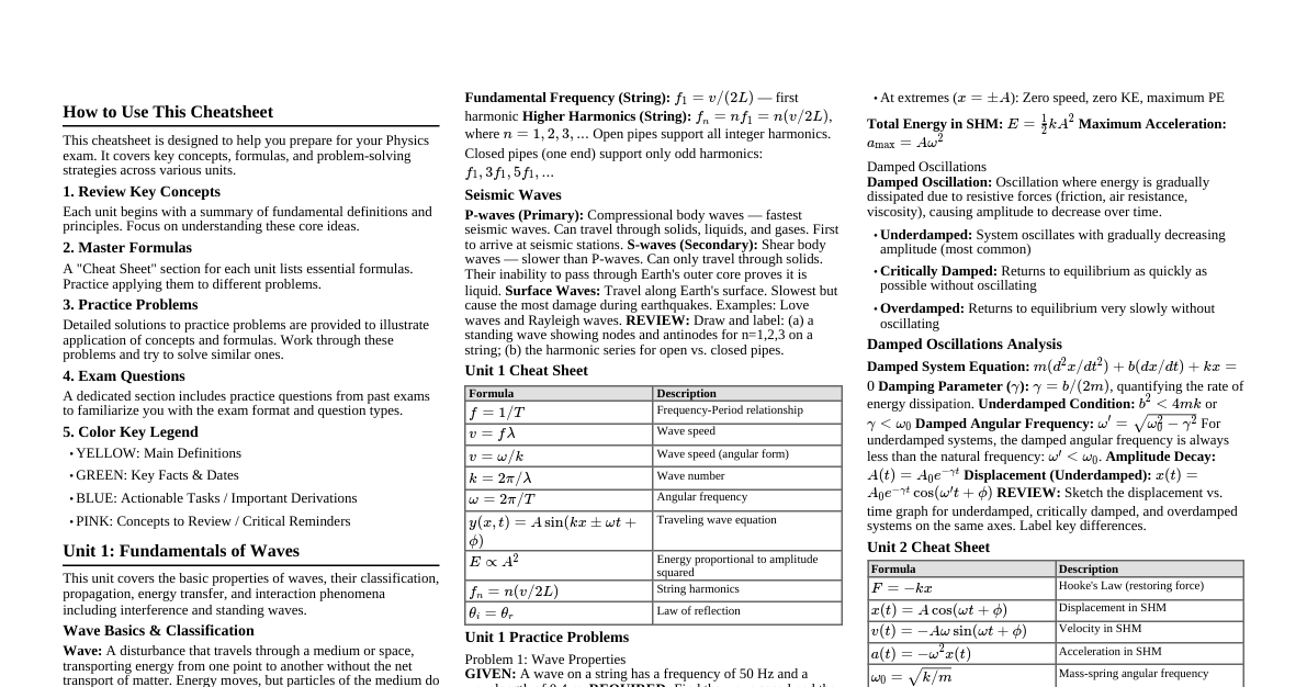
### Vector Calculus & Statics #### Coordinate Systems * **Gradient ($\nabla f$)**: * Cartesian: $\frac{\partial f}{\partial x}\mathbf{a}_x + \frac{\partial f}{\partial y}\mathbf{a}_y + \frac{\partial f}{\partial z}\mathbf{a}_z$ * Cylindrical: $\frac{\partial f}{\partial r}\mathbf{a}_r + \frac{1}{r}\frac{\partial f}{\partial \phi}\mathbf{a}_\phi + \frac{\partial f}{\partial z}\mathbf{a}_z$ * Spherical: $\frac{\partial f}{\partial R}\mathbf{a}_R + \frac{1}{R}\frac{\partial f}{\partial \theta}\mathbf{a}_\theta + \frac{1}{R\sin\theta}\frac{\partial f}{\partial \phi}\mathbf{a}_\phi$ * **Divergence ($\nabla \cdot \mathbf{A}$)**: * Cartesian: $\frac{\partial A_x}{\partial x} + \frac{\partial A_y}{\partial y} + \frac{\partial A_z}{\partial z}$ * Cylindrical: $\frac{1}{r}\frac{\partial (rA_r)}{\partial r} + \frac{1}{r}\frac{\partial A_\phi}{\partial \phi} + \frac{\partial A_z}{\partial z}$ * Spherical: $\frac{1}{R^2}\frac{\partial (R^2 A_R)}{\partial R} + \frac{1}{R\sin\theta}\frac{\partial (\sin\theta A_\theta)}{\partial \theta} + \frac{1}{R\sin\theta}\frac{\partial A_\phi}{\partial \phi}$ * **Curl ($\nabla \times \mathbf{A}$)**: * Cartesian: $(\frac{\partial A_z}{\partial y} - \frac{\partial A_y}{\partial z})\mathbf{a}_x + (\frac{\partial A_x}{\partial z} - \frac{\partial A_z}{\partial x})\mathbf{a}_y + (\frac{\partial A_y}{\partial x} - \frac{\partial A_x}{\partial y})\mathbf{a}_z$ * Cylindrical: $(\frac{1}{r}\frac{\partial A_z}{\partial \phi} - \frac{\partial A_\phi}{\partial z})\mathbf{a}_r + (\frac{\partial A_r}{\partial z} - \frac{\partial A_z}{\partial r})\mathbf{a}_\phi + \frac{1}{r}(\frac{\partial (rA_\phi)}{\partial r} - \frac{\partial A_r}{\partial \phi})\mathbf{a}_z$ * Spherical: $\frac{1}{R\sin\theta}(\frac{\partial (\sin\theta A_\phi)}{\partial \theta} - \frac{\partial A_\theta}{\partial \phi})\mathbf{a}_R + \frac{1}{R}(\frac{1}{\sin\theta}\frac{\partial A_R}{\partial \phi} - \frac{\partial (RA_\phi)}{\partial R})\mathbf{a}_\theta + \frac{1}{R}(\frac{\partial (RA_\theta)}{\partial R} - \frac{\partial A_R}{\partial \theta})\mathbf{a}_\phi$ #### Theorems * **Divergence Theorem**: $\oint_S \mathbf{A} \cdot d\mathbf{S} = \int_V (\nabla \cdot \mathbf{A}) dv$ * **Stokes’ Theorem**: $\oint_C \mathbf{A} \cdot d\mathbf{l} = \int_S (\nabla \times \mathbf{A}) \cdot d\mathbf{S}$ #### Electrostatics * **Laplace’s Equation**: $\nabla^2 V = 0$ (for charge-free regions) * **Poisson’s Equation**: $\nabla^2 V = -\frac{\rho_v}{\epsilon}$ (for regions with charge density $\rho_v$) * **Uniqueness Theorem**: A solution to Laplace’s (or Poisson’s) equation that satisfies the given boundary conditions is unique. #### Boundary Conditions | Interface | Tangential E-field | Normal D-field | Tangential H-field | Normal B-field | | :----------------------- | :-------------------------------------------------- | :-------------------------------------------------------- | :------------------------------------------------------- | :-------------------------------------------------- | | **Dielectric-Dielectric** | $E_{t1} = E_{t2}$ | $D_{n1} - D_{n2} = \rho_s$ | $H_{t1} - H_{t2} = \mathbf{J}_s \times \mathbf{a}_n$ | $B_{n1} = B_{n2}$ | | **Dielectric-Conductor** | $E_t = 0$ (inside conductor) | $D_n = \rho_s$ | $H_t = J_s$ (for perfect conductor) | $B_n = 0$ (inside perfect conductor) | *(Note: $\rho_s$ is surface charge density, $\mathbf{J}_s$ is surface current density, $\mathbf{a}_n$ is unit normal vector from medium 2 to medium 1)* * For perfect conductor: $E_t=0$, $D_n=\rho_s$, $H_t=J_s$, $B_n=0$. * For perfect dielectric: $\rho_s = 0$, $J_s = 0$. ### Maxwell’s Equations & Time-Varying Fields #### Constants * Permittivity of free space: $\epsilon_0 = 8.854 \times 10^{-12} \text{ F/m}$ * Permeability of free space: $\mu_0 = 4\pi \times 10^{-7} \text{ H/m}$ * Speed of light in free space: $c = \frac{1}{\sqrt{\mu_0\epsilon_0}} \approx 3 \times 10^8 \text{ m/s}$ #### Maxwell’s Equations | Form | Differential Form | Integral Form | | :------------- | :-------------------------------------------------- | :------------------------------------------------------------------ | | **Static Fields** | | | | Gauss's Law (E) | $\nabla \cdot \mathbf{D} = \rho_v$ | $\oint_S \mathbf{D} \cdot d\mathbf{S} = \int_V \rho_v dv = Q_{enc}$ | | Gauss's Law (M) | $\nabla \cdot \mathbf{B} = 0$ | $\oint_S \mathbf{B} \cdot d\mathbf{S} = 0$ | | Ampere's Law | $\nabla \times \mathbf{H} = \mathbf{J}$ | $\oint_C \mathbf{H} \cdot d\mathbf{l} = \int_S \mathbf{J} \cdot d\mathbf{S} = I_{enc}$ | | Faraday's Law | $\nabla \times \mathbf{E} = 0$ | $\oint_C \mathbf{E} \cdot d\mathbf{l} = 0$ | | **Time-Varying Fields** | | | | Gauss's Law (E) | $\nabla \cdot \mathbf{D} = \rho_v$ | $\oint_S \mathbf{D} \cdot d\mathbf{S} = Q_{enc}$ | | Gauss's Law (M) | $\nabla \cdot \mathbf{B} = 0$ | $\oint_S \mathbf{B} \cdot d\mathbf{S} = 0$ | | Ampere's Law | $\nabla \times \mathbf{H} = \mathbf{J} + \frac{\partial \mathbf{D}}{\partial t}$ | $\oint_C \mathbf{H} \cdot d\mathbf{l} = I_{enc} + \int_S \frac{\partial \mathbf{D}}{\partial t} \cdot d\mathbf{S}$ | | Faraday's Law | $\nabla \times \mathbf{E} = -\frac{\partial \mathbf{B}}{\partial t}$ | $\oint_C \mathbf{E} \cdot d\mathbf{l} = -\frac{\partial}{\partial t} \int_S \mathbf{B} \cdot d\mathbf{S}$ | #### Continuity Equation * **Differential Form**: $\nabla \cdot \mathbf{J} = -\frac{\partial \rho_v}{\partial t}$ * **Integral Form**: $\oint_S \mathbf{J} \cdot d\mathbf{S} = -\frac{dQ}{dt}$ * **Displacement Current Density**: $\mathbf{J}_d = \frac{\partial \mathbf{D}}{\partial t}$ #### Wave Equation Derivation Logic (for source-free, linear, isotropic, homogeneous medium) 1. Start with time-varying Maxwell's Equations (Ampere's & Faraday's): * $\nabla \times \mathbf{E} = -\mu \frac{\partial \mathbf{H}}{\partial t}$ * $\nabla \times \mathbf{H} = \epsilon \frac{\partial \mathbf{E}}{\partial t}$ (assuming $\mathbf{J}=0$) 2. Take the curl of Faraday's Law: $\nabla \times (\nabla \times \mathbf{E}) = \nabla \times (-\mu \frac{\partial \mathbf{H}}{\partial t})$ 3. Use vector identity: $\nabla \times (\nabla \times \mathbf{A}) = \nabla (\nabla \cdot \mathbf{A}) - \nabla^2 \mathbf{A}$ 4. Substitute Ampere's Law into the right side: $\nabla \times (-\mu \frac{\partial \mathbf{H}}{\partial t}) = -\mu \frac{\partial}{\partial t} (\nabla \times \mathbf{H}) = -\mu \frac{\partial}{\partial t} (\epsilon \frac{\partial \mathbf{E}}{\partial t}) = -\mu\epsilon \frac{\partial^2 \mathbf{E}}{\partial t^2}$ 5. In source-free medium, $\nabla \cdot \mathbf{D} = 0 \Rightarrow \nabla \cdot (\epsilon \mathbf{E}) = 0 \Rightarrow \nabla \cdot \mathbf{E} = 0$. 6. Combine steps 3, 4, 5: $0 - \nabla^2 \mathbf{E} = -\mu\epsilon \frac{\partial^2 \mathbf{E}}{\partial t^2}$ 7. Resulting Wave Equation for $\mathbf{E}$: $\nabla^2 \mathbf{E} - \mu\epsilon \frac{\partial^2 \mathbf{E}}{\partial t^2} = 0$ 8. Similarly for $\mathbf{H}$: $\nabla^2 \mathbf{H} - \mu\epsilon \frac{\partial^2 \mathbf{H}}{\partial t^2} = 0$ ### EM Wave Propagation #### General Propagation Constants * **Propagation Constant**: $\gamma = \alpha + j\beta = j\omega\sqrt{\mu\epsilon_c}$ where $\epsilon_c = \epsilon' - j\epsilon'' = \epsilon - j\frac{\sigma}{\omega}$ * $\alpha$ (attenuation constant, Np/m) * $\beta$ (phase constant, rad/m) * **Intrinsic Impedance**: $\eta = \sqrt{\frac{j\omega\mu}{\sigma+j\omega\epsilon}}$ #### Specific Media Formulas * **Lossless Media** ($\sigma=0$): * $\alpha = 0$ * $\beta = \omega\sqrt{\mu\epsilon}$ * $\eta = \sqrt{\frac{\mu}{\epsilon}}$ * Phase velocity $u_p = \frac{\omega}{\beta} = \frac{1}{\sqrt{\mu\epsilon}}$ * **Free Space** ($\sigma=0, \epsilon=\epsilon_0, \mu=\mu_0$): * $\alpha = 0$ * $\beta = \omega\sqrt{\mu_0\epsilon_0} = \frac{\omega}{c}$ * $\eta_0 = \sqrt{\frac{\mu_0}{\epsilon_0}} \approx 377 \Omega$ * $u_p = c \approx 3 \times 10^8 \text{ m/s}$ * **Good Conductors** ($\sigma \gg \omega\epsilon$): * $\alpha = \beta = \sqrt{\frac{\omega\mu\sigma}{2}}$ * $\eta = \sqrt{\frac{j\omega\mu}{\sigma}} = (1+j)\sqrt{\frac{\omega\mu}{2\sigma}}$ * **Skin Depth**: $\delta = \frac{1}{\alpha} = \frac{1}{\sqrt{\pi f\mu\sigma}}$ #### Power Flow * **Poynting Vector (Instantaneous)**: $\mathbf{S}(z,t) = \mathbf{E}(z,t) \times \mathbf{H}(z,t)$ (W/m$^2$) * **Average Poynting Vector**: $\mathbf{S}_{avg} = \frac{1}{2}\text{Re}(\mathbf{E}_s \times \mathbf{H}_s^*)$ (W/m$^2$) * For uniform plane wave in lossless media: $|\mathbf{S}_{avg}| = \frac{E_0^2}{2\eta}$ #### Reflection and Transmission (Normal Incidence) * **Reflection Coefficient**: $\Gamma = \frac{\eta_2 - \eta_1}{\eta_2 + \eta_1}$ * **Transmission Coefficient**: $\tau = \frac{2\eta_2}{\eta_2 + \eta_1} = 1 + \Gamma$ * **Reflected Electric Field**: $\mathbf{E}_r = \Gamma \mathbf{E}_i$ * **Transmitted Electric Field**: $\mathbf{E}_t = \tau \mathbf{E}_i$ ### Transmission Lines & Smith Chart #### Telegrapher’s Equations * $\frac{\partial V}{\partial z} = -(R + j\omega L)I$ * $\frac{\partial I}{\partial z} = -(G + j\omega C)V$ * **General Solution**: $V(z) = V_0^+ e^{-\gamma z} + V_0^- e^{\gamma z}$ $I(z) = \frac{1}{Z_0}(V_0^+ e^{-\gamma z} - V_0^- e^{\gamma z})$ where $\gamma = \sqrt{(R+j\omega L)(G+j\omega C)}$ and $Z_0 = \sqrt{\frac{R+j\omega L}{G+j\omega C}}$ #### Key Formulas * **Input Impedance**: $Z_{in}(l) = Z_0 \frac{Z_L + jZ_0 \tan(\beta l)}{Z_0 + jZ_L \tan(\beta l)}$ * For lossless line ($R=0, G=0$): $\gamma = j\beta$, $Z_0 = \sqrt{L/C}$ * **Reflection Coefficient (at load)**: $\Gamma_L = \frac{Z_L - Z_0}{Z_L + Z_0}$ * **Reflection Coefficient (at distance $l$ from load)**: $\Gamma(l) = \Gamma_L e^{j2\beta l}$ (note: often $e^{-j2\beta l}$ is used for position towards generator) * **Voltage Standing Wave Ratio (VSWR)**: $S = \frac{V_{max}}{V_{min}} = \frac{1+|\Gamma_L|}{1-|\Gamma_L|}$ * **Quarter-wave transformer**: $Z_0' = \sqrt{Z_{in} Z_L}$ #### Smith Chart 'How-to' Checklist 1. **Normalize Load Impedance**: $z_L = Z_L / Z_0$. 2. **Plot $z_L$**: Find the intersection of the $r = \text{Re}(z_L)$ circle and $x = \text{Im}(z_L)$ arc. 3. **Draw VSWR Circle**: Center at $(1,0)$, radius from center to $z_L$. 4. **Find VSWR ($S$)**: Read value at intersection of VSWR circle with positive real axis (r-axis). 5. **Determine $\Gamma_L$**: Magnitude is the distance from center to $z_L$ (normalized by chart radius). Angle is read from the 'Angle of Reflection Coefficient' scale. 6. **Move Toward Generator**: Rotate clockwise along the VSWR circle. * Distance $l$ in wavelengths corresponds to rotation angle $2\beta l = 2\pi (l/\lambda)$. * Use 'Wavelengths Toward Generator' scale. 7. **Read $z_{in}$**: Read the normalized impedance at the new position on the VSWR circle. 8. **Stub Matching**: * Move from $z_L$ along the VSWR circle to the point where the real part is 1 ($r=1$ circle). This gives $y_{in}$ or $z_{in}$. * Add a shunt stub (admittance) or series stub (impedance) to cancel the reactive part. * Refer to 'Wavelengths Toward Generator' scale to find stub position. * Determine stub length on the 'Wavelengths Toward Load' scale from short/open circuit point to desired reactive part. ### Waveguides & Antennas #### Rectangular Waveguide (dimensions $a \times b$ with $a > b$) * **Cutoff Frequency**: $f_c = \frac{1}{2\pi\sqrt{\mu\epsilon}}\sqrt{(\frac{m\pi}{a})^2 + (\frac{n\pi}{b})^2}$ * For TE/TM modes: $f_{c,mn} = \frac{1}{2\pi\sqrt{\mu\epsilon}}\sqrt{(\frac{m\pi}{a})^2 + (\frac{n\pi}{b})^2}$ * **Dominant Mode**: $TE_{10}$ (for $a > b$, $m=1, n=0$) * $f_{c,10} = \frac{1}{2a\sqrt{\mu\epsilon}}$ * **Guide Wavelength**: $\lambda_g = \frac{\lambda}{\sqrt{1 - (f_c/f)^2}}$ where $\lambda = \frac{u_p}{f} = \frac{1}{f\sqrt{\mu\epsilon}}$ * **Phase Velocity**: $u_p = \frac{u}{\sqrt{1 - (f_c/f)^2}}$ where $u = \frac{1}{\sqrt{\mu\epsilon}}$ #### Antennas * **Radiation Resistance**: $R_{rad}$ (Equivalent resistance that dissipates power equal to radiated power) * Hertzian Dipole: $R_{rad} = 80\pi^2 (\frac{dl}{\lambda})^2$ * **Gain**: $G = \frac{P_{rad}}{P_{in}} D \eta_r$ where $\eta_r$ is radiation efficiency. * **Directivity**: $D = \frac{U_{max}}{U_{avg}} = \frac{4\pi U_{max}}{P_{rad}}$ (Ratio of max radiation intensity to average) * **Far-field Expressions for Hertzian Dipole (length $dl$, current $I_0$, wavelength $\lambda$)**: * $\mathbf{E}_R = 0$ * $\mathbf{E}_\theta = j\frac{\eta I_0 dl}{2\lambda R} \sin\theta e^{-jkR} \mathbf{a}_\theta$ * $\mathbf{E}_\phi = 0$ * $\mathbf{H}_R = 0$ * $\mathbf{H}_\theta = 0$ * $\mathbf{H}_\phi = j\frac{I_0 dl}{2\lambda R} \sin\theta e^{-jkR} \mathbf{a}_\phi$ * Where $\eta$ is intrinsic impedance of medium, $k = \frac{2\pi}{\lambda}$ is wavenumber.