Data Analysis & Visualization
Cheatsheet Content
Exploratory Data Analysis (EDA) Fundamentals Classical Data Analysis vs. EDA: Classical: Focuses on formal statistical inference, hypothesis testing, confirmatory analysis. EDA: Emphasizes visualizing, summarizing, and transforming data to discover patterns, detect anomalies, and formulate hypotheses. Benefits of EDA: Uncovers underlying structure of data. Detects outliers and anomalies. Tests underlying assumptions. Develops parsimonious models. Determines optimal factor settings. Software/Libraries for EDA: Python (Pandas, Matplotlib, Seaborn, NumPy), R, SQL, Excel. Data Transformation & Reshaping Reshaping & Pivoting: Reshaping: Changing the arrangement of data (e.g., wide to long format). Pivoting: Summarizing and reorganizing data, often aggregating values based on one or more key columns. Pivot Tables/Cross-tabulations: Useful for summarizing and interpreting multi-dimensional datasets. Common Data Transformation Techniques: Scaling (Min-Max, Standardization) Log Transformation Binning/Discretization Feature Engineering Handling Missing Values (Imputation, Deletion) Categorical Encoding (One-Hot, Label Encoding) Reordering/Sorting DataFrames: Essential for structured and accessible data representation. Descriptive Statistics Mean: Average value. For numbers $x_1, ..., x_n$, mean is $\frac{1}{n} \sum_{i=1}^n x_i$. Median: Middle value when data is ordered. Less sensitive to outliers than the mean, often preferred for skewed distributions. Mode: Most frequent value. Standard Deviation ($\sigma$): Measures the spread of data around the mean. Formula: $\sigma = \sqrt{\frac{1}{n} \sum_{i=1}^n (x_i - \mu)^2}$. Interquartile Range (IQR): Range between the first quartile (Q1) and third quartile (Q3). $IQR = Q3 - Q1$. Q1 (25th percentile), Q2 (Median, 50th percentile), Q3 (75th percentile). Example: Data (2, 4, 4, 5, 6, 8, 11). Ordered: (2, 4, 4, 5, 6, 8, 11). Median (Q2) = 5. Q1 = 4. Q3 = 8. IQR = $8 - 4 = 4$. Z-score: Measures how many standard deviations an element is from the mean. $Z = \frac{X - \mu}{\sigma}$. Example: Avg length 350 pages, $\sigma = 100$ pages. Book length 80 pages. $Z = \frac{80 - 350}{100} = -2.7$. Skewness: Measures the asymmetry of the probability distribution of a real-valued random variable about its mean. Positive skewness: Tail on the right (mean > median). Negative skewness: Tail on the left (mean Kurtosis: Measures the "tailedness" of the probability distribution. Residual: The difference between the observed value and the predicted value in a statistical model ($e_i = y_i - \hat{y}_i$). Outliers Definition: Data points significantly different from other observations. Detection Techniques: Z-score (for normal distributions). IQR method: Values outside $[Q1 - 1.5 \times IQR, Q3 + 1.5 \times IQR]$. Box plots. Clustering (e.g., DBSCAN). Isolation Forests. Filtering: Removal, transformation, or capping/winsorizing. Data Visualization Purpose: Aids in understanding data, identifying patterns, communicating insights effectively. Common Types of Errors: Misleading scales, inappropriate chart types, poor color choices, cluttered designs. Matplotlib: Basic plotting library in Python. Subplots: `plt.subplots()` allows creating multiple plots within a single figure. Commands for plot customization: Title: `plt.title("Sales Data")` X-axis label: `plt.xlabel("Months")` Y-axis label: `plt.ylabel("Revenue")` Scatter Plot: `plt.scatter(x, y)`. Example: `x = [5, 7, 8]`, `y = [12, 19, 21]`. Marker: `plt.scatter(x, y, marker='s', s=100)` (squares, size 100). Density Plot (Hexbin/Contour): Useful for visualizing concentration of points in 2D data. Seaborn: High-level data visualization library based on Matplotlib. Provides a simpler interface for creating informative and attractive statistical graphics. Excellent for visualizing statistical relationships (univariate, bivariate). Example: `sns.scatterplot()`, `sns.lineplot()`, `sns.histplot()`. Histograms vs. Bar Charts: Histogram: Displays the distribution of a continuous variable (bars represent frequency within bins). Bars touch. Bar Chart: Displays frequency/counts for categorical variables. Bars typically don't touch. A histogram is a barchart in appearance but represents continuous data grouped into bins, not distinct categories. Basemap Toolkit: Used for geographic data visualization, enabling display of world boundaries and custom map projections. Style Sheets (Matplotlib/Seaborn): Improve visual appeal and consistency (e.g., 'ggplot', 'seaborn'). Variables Independent Variable: The variable that is changed or controlled in an experiment (input). Dependent Variable: The variable being tested and measured (output), whose value depends on the independent variable. Time Series Analysis Definition: Analyzing data points collected over time. Smoothing: Used to remove noise and highlight trends or cycles in time series data. Lorenz Curves: Graphical representation of income or wealth distribution, often used to illustrate inequality. Data Aggregation & Joins (Pandas) Aggregation: Combining multiple rows into a single summary row (e.g., `groupby().sum()`, `groupby().mean()`). Joins: Combining DataFrames based on common columns. Inner Join: Returns only rows with matching keys in both DataFrames. Left Outer Join: Returns all rows from the left DataFrame and matching rows from the right. If no match, fills with `NaN`. Right Outer Join: Returns all rows from the right DataFrame and matching rows from the left. If no match, fills with `NaN`. Cross Join: Returns the Cartesian product of rows, combining each row of the first DataFrame with each row of the second. Example DataFrames for Joins DataFrame 1: Students Roll no Student name Class Address 1 Adhi 10th AA 2 Abi 11th BB 3 Anu 12th CC 4 Asha 10th DD 5 Akshay 11th EE 6 Aparna 12th FF DataFrame 2: Ambition Roll no Ambition Specialization 1 Doctor Biology 2 Engineer Computer 3 IAS Social studies 4 Doctor Biology 5 Travel Explorer Geography 6 Journalist Social studies Example Sales Dataset Region Product_Category Units_Sold Revenue (₹) Discount_Applied South Electronics 120 1,80,000 Yes North Clothing 85 76,500 No East Furniture 40 1,20,000 Yes West Electronics 95 1,52,000 No South Clothing 70 65,000 No East Electronics 110 1,65,000 Yes North Furniture 35 1,05,000 Yes West Clothing 90 81,000 No South Furniture 60 1,80,000 Yes North Electronics 100 1,50,000 No Student Study Hours & Exam Scores Student Hours Studied Exam Score A 2 50 B 3 55 C 5 65 D 7 70 E 8 80 F 10 85 G 12 95 UK Male Heights (1900-1980) Year Heights in cm 1900 169.4 1910 170.9 1920 171 1930 173.9 1940 174.9 1950 176 1960 176.9 1970 177.1 1980 176.8