Physics Cheatsheet
Cheatsheet Content
### Dispersive Power and Prisms #### Dispersive Power - **Definition:** The ability of a transparent material to split white light into its constituent colors. - **Formula:** $\omega = \frac{\delta_v - \delta_r}{\delta_y}$ - $\delta_v$: Deviation for violet light - $\delta_r$: Deviation for red light - $\delta_y$: Deviation for yellow (mean) light - For a thin prism: $\omega = \frac{n_v - n_r}{n_y - 1}$ - $n_v, n_r, n_y$: Refractive indices for violet, red, and yellow light, respectively. #### Condition for Deviation without Dispersion (Achromatism) - When two thin prisms are combined such that the dispersion produced by one is nullified by the other, but deviation remains. - **Condition:** $\omega_1 \delta_{1y} + \omega_2 \delta_{2y} = 0$ - Or, for thin prisms: $(n_{1v} - n_{1r})A_1 + (n_{2v} - n_{2r})A_2 = 0$ - Where $A_1, A_2$ are the prism angles. - This implies that the net dispersion is zero, but the net deviation is generally non-zero. ### Prism Formula - **Derivation:** Consider a ray of light passing through a prism with angle $A$. - Let $i_1$ be the angle of incidence, $r_1$ the angle of refraction at the first surface. - Let $r_2$ be the angle of incidence, $i_2$ the angle of emergence at the second surface. - The angle of deviation $\delta = (i_1 - r_1) + (i_2 - r_2) = i_1 + i_2 - (r_1 + r_2)$. - From the geometry of the quadrilateral formed by the prism and the normal lines, we have $A = r_1 + r_2$. - **Therefore, the prism formula is:** $\delta = i_1 + i_2 - A$. - **At minimum deviation ($\delta_m$):** $i_1 = i_2 = i$ and $r_1 = r_2 = r$. - Then $A = 2r \Rightarrow r = A/2$. - And $\delta_m = 2i - A \Rightarrow i = (\delta_m + A)/2$. - By Snell's Law, $n = \frac{\sin i}{\sin r}$. - **Refractive index of prism:** $n = \frac{\sin((\delta_m + A)/2)}{\sin(A/2)}$. ### Transistor as an Oscillator (Ch-14) - **Principle:** An oscillator is an electronic circuit that produces a repetitive electronic signal (usually a sine wave or a square wave) without the need for an external input signal. It converts DC power into AC power. - **Working:** 1. **Feedback Loop:** A portion of the output signal is fed back to the input in phase (positive feedback). 2. **Amplification:** The transistor amplifies this feedback signal. 3. **Frequency Determination:** An LC (inductor-capacitor) tank circuit or RC (resistor-capacitor) network determines the frequency of oscillation. 4. **Sustained Oscillation:** If the loop gain (product of amplifier gain and feedback fraction) is unity or greater, and the phase shift around the loop is $0^\circ$ or $360^\circ$ (Barkhausen criterion), sustained oscillations occur. - **Labelled Diagram (Hartley Oscillator Example):** (Note: Image URL is a placeholder. A real diagram would show a transistor, tank circuit, and feedback path.) - **Components:** - Transistor (e.g., BJT or FET) as an active device for amplification. - Tank circuit (L1, L2, C) for frequency selection and phase shift. - Resistors (R1, R2, Re) for biasing. - Coupling/Bypass capacitors (Cc, Ce). - The tank circuit creates a $180^\circ$ phase shift, and the common emitter amplifier creates another $180^\circ$ phase shift, resulting in a total $360^\circ$ phase shift for positive feedback. ### Energy Bands in Solids - **Concept:** In isolated atoms, electrons occupy discrete energy levels. When atoms come together to form a solid, their atomic orbitals overlap, and according to Pauli's exclusion principle, these discrete energy levels split into a large number of closely spaced levels, forming "energy bands." - **Valence Band (VB):** The highest energy band completely or partially filled with electrons at absolute zero temperature. Electrons in this band are bound to the atoms. - **Conduction Band (CB):** The lowest energy band that is empty or partially filled with electrons. Electrons in this band are free to move and conduct electricity. - **Forbidden Energy Gap ($E_g$):** The energy difference between the top of the valence band and the bottom of the conduction band. No electron can stably exist in this gap. #### Classification of Solids based on Band Theory 1. **Conductors:** - **Band Structure:** The conduction band and valence band overlap, or the conduction band is partially filled. - **$E_g$:** Effectively zero. - **Electron Movement:** Electrons can easily move into the conduction band with very little energy, allowing for high electrical conductivity. - **Examples:** Metals (copper, silver). 2. **Semiconductors:** - **Band Structure:** A small but finite forbidden energy gap ($E_g \approx 0.5 \text{ eV to } 2 \text{ eV}$) separates the valence band from the conduction band. - **Electron Movement:** At absolute zero, they behave as insulators. At room temperature, some electrons gain enough thermal energy to jump from the valence band to the conduction band, creating holes in the valence band and free electrons in the conduction band, allowing for limited conductivity. - **Examples:** Silicon (Si, $E_g \approx 1.1 \text{ eV}$), Germanium (Ge, $E_g \approx 0.7 \text{ eV}$). 3. **Insulators:** - **Band Structure:** A very large forbidden energy gap ($E_g > 3 \text{ eV}$) exists between the valence band and the conduction band. - **Electron Movement:** Electrons require a very large amount of energy to jump from the valence band to the conduction band. Under normal conditions, virtually no electrons are in the conduction band, so they do not conduct electricity. - **Examples:** Diamond ($E_g \approx 5.5 \text{ eV}$), Glass, Wood. ### Transformer (Ch-7) - **Principle:** Mutual induction. When an alternating current (AC) flows through a primary coil, it produces a continuously changing magnetic flux in the core. This changing flux links with a secondary coil, inducing an electromotive force (EMF) in it. - **Construction:** 1. **Laminated Soft Iron Core:** Made of thin sheets of soft iron insulated from each other. This reduces eddy current losses. It provides a continuous low-reluctance path for the magnetic flux. 2. **Primary Coil ($N_p$ turns):** A coil of insulated copper wire wound around one limb of the core, connected to the AC source. 3. **Secondary Coil ($N_s$ turns):** Another coil of insulated copper wire wound around the same or another limb of the core, connected to the load. - **Working:** - Let $V_p$ be the primary voltage and $V_s$ be the secondary voltage. - Let $I_p$ be the primary current and $I_s$ be the secondary current. - According to Faraday's law of electromagnetic induction, the induced EMF in the primary coil is $E_p = -N_p \frac{d\Phi_B}{dt}$ and in the secondary coil is $E_s = -N_s \frac{d\Phi_B}{dt}$. - Assuming an ideal transformer (no flux leakage, no energy loss), $V_p \approx E_p$ and $V_s \approx E_s$. - Therefore, $\frac{V_s}{V_p} = \frac{N_s}{N_p} = k$ (transformation ratio). - For an ideal transformer, input power equals output power: $V_p I_p = V_s I_s$. - So, $\frac{I_s}{I_p} = \frac{V_p}{V_s} = \frac{N_p}{N_s} = \frac{1}{k}$. - **Step-up transformer:** $N_s > N_p \implies V_s > V_p$ (voltage increases, current decreases). - **Step-down transformer:** $N_s ### Biot-Savart Law and Magnetic Field of a Circular Coil #### Biot-Savart Law - **Statement:** It describes the magnetic field generated by a steady electric current. It states that the magnetic field $d\vec{B}$ at a point P due to a current element $d\vec{l}$ carrying current $I$ is: 1. Directly proportional to the current $I$. 2. Directly proportional to the length of the current element $d\vec{l}$. 3. Directly proportional to $\sin\theta$, where $\theta$ is the angle between $d\vec{l}$ and the position vector $\vec{r}$ from the element to the point P. 4. Inversely proportional to the square of the distance $r$ from the element to the point P. - **Mathematical Form:** $d\vec{B} = \frac{\mu_0}{4\pi} \frac{I (d\vec{l} \times \vec{r})}{r^3}$ - In magnitude: $dB = \frac{\mu_0}{4\pi} \frac{I dl \sin\theta}{r^2}$ - $\mu_0$: Permeability of free space ($4\pi \times 10^{-7} \text{ T m/A}$). #### Magnetic Field at the Axis of a Circular Coil - Consider a circular coil of radius $R$ carrying current $I$, with $N$ turns. - Let P be a point on the axis of the coil at a distance $x$ from its center. - Take a current element $d\vec{l}$ at the top of the coil. The distance from $d\vec{l}$ to P is $r = \sqrt{R^2 + x^2}$. - The angle $\theta$ between $d\vec{l}$ and $\vec{r}$ is $90^\circ$. - According to Biot-Savart law, $dB = \frac{\mu_0}{4\pi} \frac{I dl}{r^2}$. - The magnetic field $d\vec{B}$ has two components: one radial ($dB \sin\phi$) and one axial ($dB \cos\phi$). - Due to symmetry, the radial components from diametrically opposite elements cancel out. Only the axial components sum up. - $\cos\phi = \frac{R}{r} = \frac{R}{\sqrt{R^2 + x^2}}$. - Total magnetic field $B = \int dB \cos\phi = \int \frac{\mu_0}{4\pi} \frac{I dl}{r^2} \frac{R}{r}$ - $B = \frac{\mu_0 I R}{4\pi r^3} \int dl = \frac{\mu_0 I R}{4\pi (R^2 + x^2)^{3/2}} (2\pi R)$ - For $N$ turns: $B = \frac{\mu_0 N I R^2}{2(R^2 + x^2)^{3/2}}$ - **At the center of the coil (x=0):** $B_c = \frac{\mu_0 N I}{2R}$. ### Magnetic Field Due to a Bar Magnet (Broad-side-on Position) - **Broad-side-on Position (Equatorial Position):** A point P is said to be in the broad-side-on position if it lies on the perpendicular bisector of the bar magnet. - Consider a bar magnet of length $2l$ and pole strength $m$. Its magnetic dipole moment is $M = m(2l)$. - Let the point P be at a distance $r$ from the center of the magnet. - The magnetic field at P due to the North pole ($B_N$) points away from N. - The magnetic field at P due to the South pole ($B_S$) points towards S. - The magnitude of $B_N = B_S = \frac{\mu_0}{4\pi} \frac{m}{(r^2 + l^2)}$. - The components of $B_N$ and $B_S$ perpendicular to the axis of the magnet cancel out. - The components parallel to the axis of the magnet add up. Let $\theta$ be the angle between the line joining the pole to P and the perpendicular bisector. - The net magnetic field $B = B_N \cos\phi + B_S \cos\phi = 2 B_N \cos\phi$. - Where $\phi$ is the angle between the resultant field vector and the line joining the pole to P. - From the geometry, $\cos\phi = \frac{l}{\sqrt{r^2 + l^2}}$. - $B = 2 \left( \frac{\mu_0}{4\pi} \frac{m}{r^2 + l^2} \right) \frac{l}{\sqrt{r^2 + l^2}}$ - $B = \frac{\mu_0}{4\pi} \frac{2ml}{(r^2 + l^2)^{3/2}}$ - Since $M = m(2l)$, - **Magnetic field in broad-side-on position:** $B = \frac{\mu_0}{4\pi} \frac{M}{(r^2 + l^2)^{3/2}}$ - **For a short magnet ($l \ll r$):** $B = \frac{\mu_0}{4\pi} \frac{M}{r^3}$. - The direction of the magnetic field is opposite to the direction of the magnetic dipole moment (i.e., from North to South pole of the magnet). ### Electric Field Intensity and Electric Dipole #### Electric Field Intensity - **Definition:** The electric field intensity (or electric field strength) $\vec{E}$ at a point in an electric field is defined as the electrostatic force $\vec{F}$ experienced by a unit positive test charge ($q_0$) placed at that point, without disturbing the source charge. - **Formula:** $\vec{E} = \frac{\vec{F}}{q_0}$ - **Unit:** Newton per Coulomb (N/C) or Volt per meter (V/m). - It is a vector quantity, its direction is the same as the direction of the force on a positive test charge. #### Electric Field Intensity Due to an Electric Dipole - **Electric Dipole:** A system of two equal and opposite point charges ($+q$ and $-q$) separated by a small distance $2a$. - **Dipole Moment:** $\vec{p} = q(2\vec{a})$, directed from $-q$ to $+q$. ##### 1. At an Axial Point (End-on Position) - Consider a point P on the axis of the dipole at distance $r$ from its center. - Field due to $+q$: $E_{+q} = \frac{1}{4\pi\epsilon_0} \frac{q}{(r-a)^2}$, directed away from $+q$. - Field due to $-q$: $E_{-q} = \frac{1}{4\pi\epsilon_0} \frac{q}{(r+a)^2}$, directed towards $-q$. - The net electric field $\vec{E}_{axial}$ is in the direction of the dipole moment $\vec{p}$. - $E_{axial} = E_{+q} - E_{-q} = \frac{q}{4\pi\epsilon_0} \left[ \frac{1}{(r-a)^2} - \frac{1}{(r+a)^2} \right]$ - $E_{axial} = \frac{q}{4\pi\epsilon_0} \frac{(r+a)^2 - (r-a)^2}{(r^2 - a^2)^2} = \frac{q}{4\pi\epsilon_0} \frac{4ar}{(r^2 - a^2)^2}$ - Since $p = q(2a)$, - **For a short dipole ($a \ll r$):** $E_{axial} = \frac{1}{4\pi\epsilon_0} \frac{2pr}{r^4} = \frac{1}{4\pi\epsilon_0} \frac{2p}{r^3}$. ##### 2. At an Equatorial Point (Broad-side-on Position) - Consider a point P on the perpendicular bisector of the dipole at distance $r$ from its center. - Field due to $+q$: $E_{+q} = \frac{1}{4\pi\epsilon_0} \frac{q}{(r^2 + a^2)}$, directed away from $+q$. - Field due to $-q$: $E_{-q} = \frac{1}{4\pi\epsilon_0} \frac{q}{(r^2 + a^2)}$, directed towards $-q$. - Magnitudes are equal: $|E_{+q}| = |E_{-q}|$. - The vertical components cancel out due to symmetry. The horizontal components add up. - Let $\theta$ be the angle between the line joining the charge to P and the equatorial line. - The net electric field $\vec{E}_{equatorial}$ is opposite to the direction of the dipole moment $\vec{p}$. - $E_{equatorial} = 2 E_{+q} \cos\theta$. - From the geometry, $\cos\theta = \frac{a}{\sqrt{r^2 + a^2}}$. - $E_{equatorial} = 2 \frac{1}{4\pi\epsilon_0} \frac{q}{(r^2 + a^2)} \frac{a}{(r^2 + a^2)^{1/2}}$ - $E_{equatorial} = \frac{1}{4\pi\epsilon_0} \frac{2qa}{(r^2 + a^2)^{3/2}}$ - Since $p = q(2a)$, - **For a short dipole ($a \ll r$):** $E_{equatorial} = \frac{1}{4\pi\epsilon_0} \frac{p}{r^3}$. ### Half-Life and Average Life of a Radioactive Substance #### Half-Life ($T_{1/2}$) - **Definition:** The half-life of a radioactive substance is the time interval during which half of the radioactive nuclei in a given sample disintegrate. - After one half-life, 50% of the original nuclei remain. After two half-lives, 25% remain, and so on. - It is a characteristic property of a particular radioactive isotope. #### Average Life ($\tau$) - **Definition:** The average life (or mean life) of a radioactive substance is the average time for which the nuclei of a radioactive element exist before disintegrating. - It is the reciprocal of the decay constant ($\lambda$). - **Relationship:** $\tau = \frac{1}{\lambda}$ - **Relationship with Half-Life:** $\tau = \frac{T_{1/2}}{\ln(2)} \approx 1.443 T_{1/2}$ or $T_{1/2} = \tau \ln(2) \approx 0.693 \tau$. #### Disintegration Formula (Law of Radioactive Decay) - **Statement:** The rate of disintegration of radioactive nuclei at any instant is directly proportional to the number of radioactive nuclei present at that instant. - Let $N$ be the number of radioactive nuclei present at time $t$. - The rate of disintegration is $-\frac{dN}{dt}$ (negative sign indicates decrease in N). - $-\frac{dN}{dt} \propto N \implies -\frac{dN}{dt} = \lambda N$ - $\lambda$: Disintegration constant (or decay constant), characteristic of the substance. - Rearranging: $\frac{dN}{N} = -\lambda dt$ - Integrating both sides from $t=0$ (where $N=N_0$, initial number of nuclei) to time $t$ (where $N=N$): $\int_{N_0}^{N} \frac{dN}{N} = \int_{0}^{t} -\lambda dt$ $[\ln N]_{N_0}^{N} = [-\lambda t]_{0}^{t}$ $\ln N - \ln N_0 = -\lambda t$ $\ln \left( \frac{N}{N_0} \right) = -\lambda t$ - Taking exponential on both sides: **$N = N_0 e^{-\lambda t}$** - This is the disintegration formula, showing the exponential decay of radioactive nuclei over time. ### Capacitance and Stored Energy in a Parallel Plate Capacitor #### Capacitance of a Capacitor - **Definition:** The capacitance ($C$) of a capacitor is a measure of its ability to store electric charge. It is defined as the ratio of the magnitude of the charge ($Q$) stored on either conductor plate to the potential difference ($V$) between the plates. - **Formula:** $C = \frac{Q}{V}$ - **Unit:** Farad (F). 1 Farad = 1 Coulomb/Volt. #### Expression for Stored Energy in a Parallel Plate Capacitor - When a capacitor is charged, work is done by the external source in transferring charge from one plate to another against the electrostatic forces. This work is stored as potential energy in the electric field between the plates. - Consider a capacitor with capacitance $C$. If at some instant, charge on the plates is $q$ and potential difference is $v = q/C$. - The small amount of work done $dW$ in transferring an additional small charge $dq$ is: $dW = v dq = \frac{q}{C} dq$ - To charge the capacitor from $0$ to a final charge $Q$, the total work done (stored energy $U$) is: $U = \int_0^Q \frac{q}{C} dq = \frac{1}{C} \left[ \frac{q^2}{2} \right]_0^Q$ **$U = \frac{1}{2} \frac{Q^2}{C}$** - Using $Q = CV$, we can express the energy in alternative forms: **$U = \frac{1}{2} C V^2$** **$U = \frac{1}{2} Q V$** #### Energy Density Between Plates of a Capacitor - For a parallel plate capacitor, let $A$ be the area of each plate and $d$ be the distance between them. - Capacitance $C = \frac{\epsilon_0 A}{d}$ (for vacuum/air between plates). - The potential difference $V = Ed$, where $E$ is the electric field between the plates. - Substitute these into the energy formula $U = \frac{1}{2} C V^2$: $U = \frac{1}{2} \left( \frac{\epsilon_0 A}{d} \right) (Ed)^2$ $U = \frac{1}{2} \frac{\epsilon_0 A}{d} E^2 d^2$ $U = \frac{1}{2} \epsilon_0 A d E^2$ - The volume between the plates is $Volume = Ad$. - **Energy density ($u$)** is the energy stored per unit volume: $u = \frac{U}{Volume}$ $u = \frac{\frac{1}{2} \epsilon_0 A d E^2}{Ad}$ **$u = \frac{1}{2} \epsilon_0 E^2$** - This shows that the energy density depends only on the electric field strength and the permittivity of the medium, not on the dimensions of the capacitor. ### Bohr's Atomic Model and Hydrogen Spectrum #### Postulates of Bohr's Atomic Model (for Hydrogen-like atoms) 1. **Quantized Orbits:** Electrons revolve around the nucleus in certain stable, non-radiating circular orbits, called stationary orbits. These orbits have definite energy. 2. **Quantization of Angular Momentum:** An electron can revolve only in those orbits for which its angular momentum is an integral multiple of $\frac{h}{2\pi}$ (where $h$ is Planck's constant). - $L = mvr = n \frac{h}{2\pi}$, where $n = 1, 2, 3, ...$ (principal quantum number). 3. **Energy Transitions (Quantum Jumps):** An electron does not radiate energy while in a stationary orbit. Energy is emitted or absorbed only when an electron jumps from one stationary orbit to another. - When an electron jumps from a higher energy orbit ($E_2$) to a lower energy orbit ($E_1$), it emits a photon with energy $h\nu = E_2 - E_1$. - When an electron absorbs a photon of energy $h\nu$, it jumps from a lower energy orbit ($E_1$) to a higher energy orbit ($E_2$). #### Explanation of Hydrogen Spectrum on the Basis of Bohr's Theory - Bohr's theory successfully explained the line spectrum of hydrogen. - **Energy of an Electron in the $n$-th Orbit:** $E_n = -\frac{me^4}{8\epsilon_0^2 h^2 n^2} = -\frac{13.6}{n^2} \text{ eV}$ - When an electron jumps from an initial higher energy orbit ($n_i$) to a final lower energy orbit ($n_f$), it emits a photon. - The energy of the emitted photon is $h\nu = E_{n_i} - E_{n_f}$. - $\frac{hc}{\lambda} = E_{n_i} - E_{n_f} = -13.6 \left( \frac{1}{n_i^2} - \frac{1}{n_f^2} \right) \text{ eV}$ - $\frac{1}{\lambda} = R \left( \frac{1}{n_f^2} - \frac{1}{n_i^2} \right)$ - $R$ is the Rydberg constant, $R = \frac{me^4}{8\epsilon_0^2 ch^3} \approx 1.097 \times 10^7 \text{ m}^{-1}$. - **Spectral Series:** Different series correspond to different final orbits ($n_f$): 1. **Lyman Series:** $n_f = 1$, $n_i = 2, 3, 4, ...$ (Ultraviolet region) - $\frac{1}{\lambda} = R \left( \frac{1}{1^2} - \frac{1}{n_i^2} \right)$ 2. **Balmer Series:** $n_f = 2$, $n_i = 3, 4, 5, ...$ (Visible region) - $\frac{1}{\lambda} = R \left( \frac{1}{2^2} - \frac{1}{n_i^2} \right)$ 3. **Paschen Series:** $n_f = 3$, $n_i = 4, 5, 6, ...$ (Infrared region) - $\frac{1}{\lambda} = R \left( \frac{1}{3^2} - \frac{1}{n_i^2} \right)$ 4. **Brackett Series:** $n_f = 4$, $n_i = 5, 6, 7, ...$ (Infrared region) - $\frac{1}{\lambda} = R \left( \frac{1}{4^2} - \frac{1}{n_i^2} \right)$ 5. **Pfund Series:** $n_f = 5$, $n_i = 6, 7, 8, ...$ (Infrared region) - $\frac{1}{\lambda} = R \left( \frac{1}{5^2} - \frac{1}{n_i^2} \right)$ - Bohr's theory accurately predicted the wavelengths of these spectral lines, thus providing strong evidence for the quantization of energy levels in atoms.