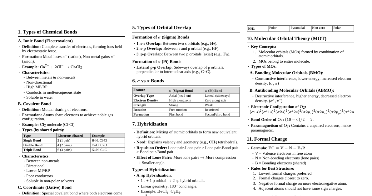
Chemical Bonding Essentials

Cheatsheet Content

1.0 INTRODUCTION TO CHEMICAL BONDING Atoms combine to form molecules or ionic compounds to achieve a more stable, lower energy state. This fundamental principle drives all chemical interactions. This stability is primarily achieved by attaining a noble gas electron configuration (octet rule) or by arranging electrons in a way that minimizes the overall potential energy of the system through strong attractive forces. A chemical bond is defined as the strong attractive force that holds two or more atoms or ions together in a stable chemical entity (molecule, ion, or crystal lattice). Bond formation is an inherently exothermic process; energy is released when atoms form bonds, indicating that the resulting compound is more stable and at a lower energy state than the separated atoms. The magnitude of this released energy is known as the bond energy. The strength of a chemical bond is inversely proportional to its potential energy. A lower potential energy corresponds to a stronger, more stable bond. 1.1 Classification of Chemical Bonds Strong Bonds (Intramolecular, Interatomic): These bonds occur *within* molecules or ionic lattices, involving direct electron interactions between atoms. They are characterized by significant electron redistribution (either transfer or sharing) and possess high bond energies, typically ranging from $200 \text{ kJ/mol}$ to over $800 \text{ kJ/mol}$. These bonds are responsible for the fundamental chemical identity and structure of substances. Ionic Bond: Formed by the complete transfer of one or more valence electrons from a metal atom (low ionization energy) to a non-metal atom (high electron affinity), resulting in electrostatic attraction between oppositely charged ions. Covalent Bond: Formed by the mutual sharing of one or more pairs of valence electrons between two non-metal atoms, leading to a stable electron configuration (often an octet). Co-ordinate (Dative) Bond: A specific type of covalent bond where both shared electrons in the bond originate from only one of the participating atoms. Once formed, it behaves identically to a regular covalent bond. Metallic Bond: Found in solid metals and alloys, characterized by a "sea" of delocalized valence electrons shared among a lattice of positively charged metal ions. This model explains the characteristic properties of metals like conductivity and malleability. Weak Bonds (Intermolecular Forces): These are attractive forces that exist *between* molecules. They are significantly weaker than strong chemical bonds, with bond energies typically in the range of $2 \text{ kJ/mol}$ to $40 \text{ kJ/mol}$. Intermolecular forces (IMFs) do not involve electron transfer or sharing between atoms to form new chemical species but rather represent attractions between existing molecules. They are crucial in determining the physical properties of substances such as melting points, boiling points, viscosity, surface tension, and solubility. Hydrogen Bond: A particularly strong type of dipole-dipole interaction involving a hydrogen atom bonded to a highly electronegative atom (F, O, or N) and attracted to another F, O, or N atom. Van der Waals Forces: A collective term encompassing all other types of weak intermolecular forces. London Dispersion Forces (LDFs) / Induced Dipole-Induced Dipole Forces: Present in all molecules, arising from temporary, instantaneous dipoles due to random electron movement. Dipole-Dipole Forces: Occur between molecules with permanent dipoles (polar molecules). Dipole-Induced Dipole Forces: Occur between a polar molecule and a non-polar molecule, where the polar molecule induces a temporary dipole in the non-polar one. 1.2 Driving Forces for Chemical Combination Achieving Minimum Energy (Potential Energy Minimization): As two isolated atoms approach each other, a complex interplay of forces occurs: Attractive forces: Between the nucleus of one atom and the electron cloud of the other atom. These forces lead to a decrease in potential energy. Repulsive forces: Between the nuclei of both atoms (due to positive charges) and between the electron clouds of both atoms (due to negative charges). These forces lead to an increase in potential energy. A stable chemical bond forms *only if* the net attractive forces are stronger than the repulsive forces. This results in a net decrease in the potential energy of the system, indicating increased stability. The bond length of a stable molecule corresponds to the internuclear distance at which the total potential energy of the system is at its absolute minimum. At this optimal distance, the attractive and repulsive forces are balanced. Internuclear distance Potential energy (kJ/mole)→ Bond Energy 0 Achieving Noble Gas Configuration (The Octet Rule): This principle, primarily associated with Kossel and Lewis, posits that atoms tend to react in ways that allow them to attain the electron configuration of the nearest noble gas. This usually means having eight electrons in their outermost valence shell (an octet), which is a particularly stable configuration. For the lightest elements, specifically hydrogen (H) and lithium (Li), achieving a duplet ($1s^2$) configuration (like helium) is the goal. Crucially, only the valence electrons (electrons located in the outermost electron shell) are involved in chemical bonding. These are often visually represented using Lewis dot symbols. Atoms can achieve this stable configuration through: Electron transfer: Leading to the formation of ionic bonds. Electron sharing: Leading to the formation of covalent bonds. 2.0 VALENCY & OCTET RULE 2.1 Valency Valency is a measure of the combining power of an element. It indicates the number of chemical bonds an atom can typically form. Historical/Classical Concept: Initially defined by the number of hydrogen atoms an element could combine with (e.g., in $HCl$, Cl has a valency of 1; in $H_2O$, O has a valency of 2) or double the number of oxygen atoms. This concept was purely empirical. Modern Concept (Electronic Valency): Based on the electronic configuration of atoms and their tendency to achieve noble gas configurations. For main group elements in Groups 1, 2, 13, and 14: Valency is generally equal to the number of valence electrons. For example, sodium (Na, Group 1) has 1 valence electron and a valency of 1. Carbon (C, Group 14) has 4 valence electrons and a valency of 4. For main group elements in Groups 15, 16, 17, and 18: Valency is often calculated as $8 - \text{Number of valence electrons}$. This represents the number of electrons an atom needs to gain or share to complete an octet. For example, chlorine (Cl, Group 17) has 7 valence electrons and a typical valency of $8-7=1$. Elements within the same group of the periodic table generally exhibit similar valencies because they share the same number of valence shell electrons and thus similar chemical behaviors. 2.2 Kossel-Lewis Approach & Octet Rule Lewis Dot Structures (or Lewis Electron Dot Structures): A simplified representation of the valence electrons of an atom as dots placed around the element's symbol. These structures are fundamental for understanding the Kossel-Lewis approach. The central tenet of this approach is that atoms achieve chemical stability by attaining an electron configuration identical to that of a noble gas. This is primarily accomplished by: Electron Transfer: Atoms with low ionization energies (metals) transfer electrons to atoms with high electron affinities (non-metals), forming ions that are then held together by electrostatic forces (ionic bonding). Electron Sharing: Atoms (typically non-metals) share electrons to complete their valence shells, forming covalent bonds. Each shared pair of electrons contributes to the octet (or duplet) of both participating atoms. 2.3 Exceptions to the Octet Rule While the octet rule serves as an excellent guiding principle, it is not universally applicable, and several classes of exceptions exist: 1. Incomplete Octet Molecules (Electron-Deficient Compounds): These are molecules where the central atom, even after forming all its bonds, has fewer than eight electrons in its valence shell. Such compounds are often highly reactive and function as Lewis acids, readily accepting electron pairs. Examples: $BF_3$: Boron (B) forms three bonds with fluorine, resulting in only 6 valence electrons around B. $BeCl_2$: Beryllium (Be) forms two bonds with chlorine, leaving only 4 valence electrons around Be. $AlCl_3$: Aluminum (Al) forms three bonds with chlorine, resulting in 6 valence electrons around Al. Some elements in Group 13 (like Boron and Aluminum) commonly form compounds with incomplete octets. 2. Expanded Octet Molecules (Hypervalent Compounds): Elements in the third period and beyond (e.g., Phosphorus, Sulfur, Chlorine, Bromine, Iodine, Xenon) can accommodate more than eight electrons in their valence shell. This capacity arises from the availability of vacant, low-energy d-orbitals that can participate in bonding. Examples: $PCl_5$: Phosphorus (P) forms five bonds, placing 10 electrons in its valence shell. $SF_6$: Sulfur (S) forms six bonds, resulting in 12 electrons around S. $IF_7$: Iodine (I) forms seven bonds, leading to 14 electrons around I. $H_2SO_4$: Sulfur in sulfuric acid often shows an expanded octet. 3. Odd-Electron Molecules (Radicals): These are molecules that possess an odd total number of valence electrons. Consequently, it's impossible for all atoms in such molecules to satisfy the octet rule. The central atom often ends up with an odd number of electrons. Odd-electron molecules are typically highly reactive and are characterized by paramagnetism (they are attracted to a magnetic field due to the presence of unpaired electrons). Examples: $NO$ (nitric oxide, with 11 total valence electrons, N has 7), $NO_2$ (nitrogen dioxide, with 17 total valence electrons, N has 7), $ClO_2$. 4. Other Limitations and Inadequacies of the Octet Theory: Molecular Geometry: The octet rule offers no explanation for the three-dimensional shapes of molecules. For example, it doesn't explain why water ($H_2O$) is bent while carbon dioxide ($CO_2$) is linear, even though both satisfy the octet rule. Relative Stability and Bond Energies: It cannot quantitatively predict the relative stability of different molecules or the precise values of bond energies. Noble Gas Compounds: The theory was based on the assumed inertness of noble gases. However, compounds like xenon difluoride ($XeF_2$) and krypton difluoride ($KrF_2$) exist, challenging the notion that noble gases never form bonds. 3.0 COVALENT BONDING A covalent bond is formed by the mutual sharing of one or more pairs of valence electrons between two atoms. This type of bonding predominantly occurs between non-metal atoms (or between a non-metal and a metalloid) that have similar electronegativities, meaning neither atom is strong enough to completely pull electrons away from the other. Each shared electron pair contributes simultaneously to the valence shell of both participating atoms, effectively allowing both atoms to achieve a more stable electron configuration, often resembling a noble gas. The shared electrons are typically localized between the two bonded atoms, though in some cases (resonance), they can be delocalized over multiple atoms. The electrons involved in a shared pair must have opposite spins (according to Pauli's exclusion principle). Covalent bonds are categorized based on the number of electron pairs shared: Single bond (-): Involves the sharing of 2 electrons (1 shared pair) between two atoms. Example: The $H-H$ bond in molecular hydrogen ($H_2$). Double bond (=): Involves the sharing of 4 electrons (2 shared pairs) between two atoms. Example: The $O=O$ bond in molecular oxygen ($O_2$). Triple bond ($\equiv$): Involves the sharing of 6 electrons (3 shared pairs) between two atoms. Example: The $N\equiv N$ bond in molecular nitrogen ($N_2$). 3.1 Orbital Concept of Covalent Bond (Valence Bond Theory - VBT) The Valence Bond Theory (VBT), developed by Heitler, London, Pauling, and Slater, provides a quantum mechanical explanation for covalent bonding. According to VBT, a covalent bond forms when two atomic orbitals, each containing a single unpaired electron, overlap. The overlapping region is then occupied by these two electrons, which must have opposite spins. The extent of overlap between the atomic orbitals is directly related to the strength of the resulting covalent bond. Greater overlap leads to a stronger bond, which corresponds to a lower potential energy for the molecule. A key aspect of VBT is its emphasis on the directional nature of covalent bonds. Atomic orbitals (especially p and d orbitals) have specific spatial orientations. When these orbitals overlap, they do so in specific directions that maximize overlap, thereby dictating the three-dimensional geometry of the molecule. 3.2 Types of Overlap and Covalent Bonds Sigma ($\sigma$) Bond: Formation: A $\sigma$ bond is formed by the direct, head-on (or axial) overlap of atomic orbitals along the internuclear axis. This means the electron density is concentrated symmetrically around the line connecting the two nuclei. Strength: $\sigma$ bonds are generally the strongest type of covalent bond due to the extensive and direct overlap of orbitals, which maximizes electron density directly between the nuclei. Characteristics: Electron density is cylindrically symmetrical about the internuclear axis. Rotation around a $\sigma$ bond is generally free (unless sterically hindered or part of a rigid ring structure). Types of Overlap: $s-s$ overlap: Occurs between two $s$ orbitals (e.g., in $H-H$ bond of $H_2$). $s-p$ overlap: Occurs between an $s$ orbital and a $p$ orbital (e.g., in $H-F$ bond of $HF$). $p-p$ axial overlap: Occurs between two $p$ orbitals oriented head-on along the internuclear axis (e.g., in $Cl-Cl$ bond of $Cl_2$). Rule: Only one $\sigma$ bond can exist between any two atoms. All single bonds are $\sigma$ bonds. In multiple bonds, one bond is always a $\sigma$ bond. Pi ($\pi$) Bond: Formation: A $\pi$ bond is formed by the lateral (sideways) overlap of parallel atomic orbitals (typically $p$ orbitals, but sometimes $d$ orbitals). The electron density is concentrated above and below the internuclear axis, with a nodal plane along the axis. Strength: $\pi$ bonds are generally weaker than $\sigma$ bonds because the sideways overlap is less effective, resulting in less electron density concentrated directly between the nuclei. Characteristics: $\pi$ bonds are non-rotational; rotation around a $\pi$ bond would break the bond, requiring significant energy. This restricted rotation is responsible for cis-trans isomerism. Rule: $\pi$ bonds are always formed in conjunction with a $\sigma$ bond. A double bond consists of one $\sigma$ bond and one $\pi$ bond (e.g., $C=C$). A triple bond consists of one $\sigma$ bond and two $\pi$ bonds (e.g., $C\equiv C$). Relative Bond Strengths (based on orbital overlap): For $\sigma$ bonds involving the same principal quantum number: $p-p \text{ (axial)} > s-p \text{ (axial)} > s-s \text{ (axial)}$. This is because $p$ orbitals are more directional than $s$ orbitals, leading to more effective overlap. Bond strength also depends on the principal quantum number ($n$) of the orbitals involved: Smaller $n$ (meaning smaller, more compact orbitals) generally leads to better overlap and stronger bonds. For example, a $1s-1s$ overlap is typically stronger than a $2s-2s$ overlap. While individual $\pi$ bonds are weaker than individual $\sigma$ bonds, the presence of multiple bonds (double or triple) makes the overall bond between two atoms stronger and shorter than a single bond, due to the cumulative strength of both $\sigma$ and $\pi$ components. 3.3 Variable Valency in Covalent Compounds Many elements, particularly those located in Period 3 and subsequent periods of the periodic table, exhibit variable valencies (i.e., they can form different numbers of covalent bonds). This phenomenon is primarily attributed to the availability of vacant d-orbitals in their valence shell. Mechanism: Electrons from paired orbitals (either $s$ or $p$ orbitals) can be promoted (excited) to these vacant d-orbitals. This promotion increases the number of unpaired electrons available for bonding, thereby increasing the element's covalency. This process requires an input of energy, known as promotion energy or excitation energy. Example: Phosphorus (P, Group 15, Period 3): Ground state: The valence electron configuration is $3s^2 3p^3$. This provides three unpaired electrons in the $3p$ orbitals, leading to a typical covalency of 3 (e.g., in $PCl_3$). First excited state: One electron from the $3s$ orbital is promoted to a vacant $3d$ orbital. The configuration becomes $3s^1 3p^3 3d^1$. This now provides five unpaired electrons, allowing phosphorus to exhibit a covalency of 5 (e.g., in $PCl_5$). Example: Sulfur (S, Group 16, Period 3): Ground state: Valence electron configuration is $3s^2 3p^4$. This provides two unpaired electrons in the $3p$ orbitals, leading to a covalency of 2 (e.g., in $H_2S$, $SCl_2$). First excited state: One electron from a $3p$ orbital is promoted to a vacant $3d$ orbital. The configuration becomes $3s^2 3p^3 3d^1$. This provides four unpaired electrons, allowing sulfur to exhibit a covalency of 4 (e.g., in $SF_4$). Second excited state: One electron from the $3s$ orbital is promoted to a vacant $3d$ orbital. The configuration becomes $3s^1 3p^3 3d^2$. This provides six unpaired electrons, allowing sulfur to exhibit a covalency of 6 (e.g., in $SF_6$). Limitation for Period 2 Elements: Elements in the second period (e.g., Nitrogen, Oxygen, Fluorine) cannot expand their octet because they do not possess any d-orbitals in their valence shell ($n=2$, so only $2s$ and $2p$ orbitals exist, no $2d$). This is why $NCl_5$ does not exist, whereas $PCl_5$ is a stable compound. 4.0 HYBRIDISATION The concept of hybridization was initially proposed by Linus Pauling to reconcile the observed geometries and equivalent bond characteristics of molecules (which VBT couldn't fully explain with pure atomic orbitals) with quantum mechanical principles. Definition: Hybridization is a theoretical concept describing the hypothetical process of mixing atomic orbitals of slightly different energies (but belonging to the same atom) to form an equal number of new, identical hybrid orbitals. These new hybrid orbitals are degenerate (have equal energy), have identical shapes, and are symmetrically oriented in space. This process primarily occurs on the central atom within a molecule. Hybridization is considered a conceptual process that occurs *before* the actual formation of chemical bonds. Hybrid orbitals are generally more directional than pure atomic orbitals. This enhanced directionality allows them to achieve more effective overlap with orbitals from other atoms, leading to the formation of stronger $\sigma$ bonds. The spatial arrangement of these newly formed hybrid orbitals is crucial as it dictates the three-dimensional geometry of the molecule, by minimizing electron pair repulsion. 4.1 Important Conditions for Hybridisation Valence Shell Orbitals: Only atomic orbitals belonging to the valence shell of an atom participate in hybridization. Inner shell orbitals are too stable and deeply held to mix. Comparable Energy: The atomic orbitals undergoing hybridization must have energies that are reasonably close to each other. For instance, $2s$ and $2p$ orbitals can hybridize, but $1s$ and $2p$ orbitals usually do not. Electron Promotion Not Always Essential: While electron promotion (e.g., from $s$ to $d$ orbital) often precedes hybridization to create more unpaired electrons for bonding, it is not always a prerequisite. For example, in $NH_3$ and $H_2O$, hybridization occurs without electron promotion, involving originally paired electrons (which become lone pairs in the hybrid orbitals). Participation of Different Electron States: Not only half-filled atomic orbitals (which form bonds) but also completely filled atomic orbitals (which become lone pairs in hybrid orbitals) and even empty atomic orbitals (which can become vacant hybrid orbitals for accepting electron pairs in coordinate bonds) can participate in hybridization. 4.2 Determining Hybridization State Method 1 (Counting Electron Domains / Steric Number): This is the most intuitive and widely used method. Count the total number of electron domains (regions of electron density) around the central atom. Each $\sigma$ bond (single, double, or triple bond counts as one $\sigma$ bond) and each lone pair of electrons counts as one electron domain. 2 electron domains $\rightarrow$ $sp$ hybridization 3 electron domains $\rightarrow$ $sp^2$ hybridization 4 electron domains $\rightarrow$ $sp^3$ hybridization 5 electron domains $\rightarrow$ $sp^3d$ hybridization 6 electron domains $\rightarrow$ $sp^3d^2$ hybridization 7 electron domains $\rightarrow$ $sp^3d^3$ hybridization Method 2 (Formula for Steric Number, SN): This method is particularly useful for polyatomic ions or complex molecules. Steric Number (SN) = $1/2 (\text{V} + \text{M} - \text{C} + \text{A})$ V: Represents the number of valence electrons of the central atom. M: Represents the number of monovalent atoms (like Hydrogen (H) or halogens such as F, Cl, Br, I) directly attached to the central atom. These atoms form only one $\sigma$ bond. C: Represents the cationic charge (if the molecule is a cation). This value is subtracted from the total because cationic charge implies fewer electrons. A: Represents the anionic charge (if the molecule is an anion). This value is added to the total because anionic charge implies more electrons. The calculated Steric Number directly corresponds to the number of electron domains, which then determines the hybridization type (e.g., SN=4 implies $sp^3$ hybridization). 4.3 Types of Hybridization and Resulting Molecular Geometry $sp$ Hybridization: Formation: Involves the mixing of one $s$ atomic orbital and one $p$ atomic orbital to produce two new $sp$ hybrid orbitals. Geometry: These two $sp$ hybrid orbitals orient themselves $180^\circ$ apart from each other to minimize repulsion. This results in a Linear electron geometry and molecular shape. Bond Angle: $180^\circ$. % s-character: 50%, % p-character: 50%. (High s-character makes bonds stronger and shorter). Examples: $BeCl_2$, $CO_2$, $C_2H_2$ (acetylene, each carbon atom is $sp$ hybridized). $sp^2$ Hybridization: Formation: Involves the mixing of one $s$ atomic orbital and two $p$ atomic orbitals to produce three new $sp^2$ hybrid orbitals. One $p$ orbital remains unhybridized. Geometry: These three $sp^2$ hybrid orbitals lie in a single plane and are oriented $120^\circ$ apart, pointing towards the corners of an equilateral triangle. This results in a Trigonal Planar electron geometry. Bond Angle: $120^\circ$. % s-character: 33.3%, % p-character: 66.7%. Examples: $BF_3$, $C_2H_4$ (ethene, each carbon atom is $sp^2$ hybridized), $NO_3^-$ (nitrate ion), $SO_3$. With one lone pair: If one of the electron domains is a lone pair (e.g., in $SO_2$), the electron geometry remains trigonal planar, but the molecular shape becomes Bent or Angular, with a bond angle slightly less than $120^\circ$ due to LP-BP repulsion. $sp^3$ Hybridization: Formation: Involves the mixing of one $s$ atomic orbital and all three $p$ atomic orbitals to produce four new $sp^3$ hybrid orbitals. Geometry: These four $sp^3$ hybrid orbitals are directed towards the corners of a regular tetrahedron, maximizing their separation. This results in a Tetrahedral electron geometry. Bond Angle: The ideal bond angle is $109.5^\circ$ ($109^\circ 28'$). % s-character: 25%, % p-character: 75%. Examples: $CH_4$ (methane), $CCl_4$ (carbon tetrachloride), $NH_4^+$ (ammonium ion), $H_2O$ (water), $NH_3$ (ammonia). With one lone pair: If one of the four electron domains is a lone pair (e.g., in $NH_3$), the electron geometry is tetrahedral, but the molecular shape becomes Trigonal Pyramidal. The LP-BP repulsion reduces the bond angle to approximately $107^\circ$. With two lone pairs: If two of the four electron domains are lone pairs (e.g., in $H_2O$), the electron geometry is tetrahedral, but the molecular shape becomes Bent or Angular. The LP-LP and LP-BP repulsions further reduce the bond angle to approximately $104.5^\circ$. $sp^3d$ Hybridization: Formation: Involves the mixing of one $s$, three $p$, and one $d$ orbital (specifically the $d_{z^2}$ orbital, as it aligns along the bond axis) to form five $sp^3d$ hybrid orbitals. This hybridization is characteristic of central atoms in Period 3 and beyond. Geometry: The five hybrid orbitals adopt a Trigonal Bipyramidal (TBP) electron geometry. Three orbitals lie in an equatorial plane ($120^\circ$ apart), and two are axial (perpendicular to the equatorial plane, $90^\circ$ to the equatorial bonds). Bond Angles: $120^\circ$ (equatorial positions) and $90^\circ$ (axial positions). Axial bonds are typically slightly longer and weaker than equatorial bonds due to greater repulsive interactions from the equatorial bond pairs. Examples: $PCl_5$ (phosphorus pentachloride), $PF_5$. With one lone pair: If one of the five electron domains is a lone pair (e.g., in $SF_4$), the electron geometry is TBP, but the molecular shape is See-saw. The lone pair preferentially occupies an equatorial position to minimize $90^\circ$ repulsions. With two lone pairs: If two electron domains are lone pairs (e.g., in $ClF_3$), the molecular shape is T-shaped. Both lone pairs occupy equatorial positions. With three lone pairs: If three electron domains are lone pairs (e.g., in $XeF_2$, $I_3^-$), the molecular shape is Linear. All three lone pairs occupy the equatorial positions, and the two axial atoms form a linear arrangement. $sp^3d^2$ Hybridization: Formation: Involves the mixing of one $s$, three $p$, and two $d$ orbitals (specifically the $d_{z^2}$ and $d_{x^2-y^2}$ orbitals) to form six $sp^3d^2$ hybrid orbitals. Also characteristic of central atoms in Period 3 and beyond. Geometry: The six hybrid orbitals are directed towards the corners of a regular octahedron. This results in an Octahedral electron geometry. Bond Angles: All adjacent bond angles are $90^\circ$. Examples: $SF_6$ (sulfur hexafluoride), $[AlF_6]^{3-}$ (hexafluoroaluminate ion). With one lone pair: If one of the six electron domains is a lone pair (e.g., in $BrF_5$, $XeOF_4$), the electron geometry is octahedral, but the molecular shape becomes Square Pyramidal. The lone pair can be placed at any position, as all positions are equivalent in an ideal octahedron. With two lone pairs: If two electron domains are lone pairs (e.g., in $XeF_4$, $ICl_4^-$), the electron geometry is octahedral, but the molecular shape becomes Square Planar. The two lone pairs always occupy opposite positions (trans) to minimize LP-LP repulsion. $sp^3d^3$ Hybridization: Formation: Involves the mixing of one $s$, three $p$, and three $d$ orbitals to form seven $sp^3d^3$ hybrid orbitals. Geometry: These seven hybrid orbitals adopt a Pentagonal Bipyramidal electron geometry. Five orbitals lie in an equatorial plane ($72^\circ$ apart), and two are axial ($90^\circ$ to the equatorial plane). Bond Angles: $72^\circ$ (equatorial positions) and $90^\circ$ (axial positions). Examples: $IF_7$ (iodine heptafluoride). 5.0 VSEPR THEORY (VALENCE SHELL ELECTRON PAIR REPULSION) The VSEPR (Valence Shell Electron Pair Repulsion) theory, developed by Sidgwick, Powell, Gillespie, and Nyholm, provides a straightforward and highly effective model for predicting the three-dimensional geometry of molecules and polyatomic ions. The core principle of VSEPR theory is that electron pairs (both bonding pairs, forming covalent bonds, and non-bonding pairs, or lone pairs) in the valence shell of a central atom will arrange themselves in space to be as far apart as possible. This arrangement minimizes the electrostatic repulsion between these negatively charged electron domains. This spatial arrangement of electron domains dictates the *electron geometry* around the central atom. The *molecular shape* (or molecular geometry) is then determined by considering only the positions of the atoms, effectively ignoring the lone pairs (though their repulsive influence is still considered). Key Postulates of VSEPR Theory: Electron Domain Repulsion: The shape of a molecule is determined by the number of electron domains (regions of electron density) around the central atom. These electron domains repel each other. Minimization of Repulsion: To achieve maximum stability, electron domains will arrange themselves in space to maximize the distance between them, thereby minimizing their mutual repulsion. Order of Repulsion: The repulsive forces between different types of electron domains follow a specific order: Lone pair-Lone pair (LP-LP) repulsion is strongest. Lone pair-Bond pair (LP-BP) repulsion is intermediate. Bond pair-Bond pair (BP-BP) repulsion is weakest. This order explains why actual bond angles in molecules with lone pairs are often slightly smaller than the ideal bond angles predicted by electron geometry alone (e.g., $H_2O$ has a smaller bond angle than $CH_4$). Valence Shell as a Sphere: The valence shell of the central atom is considered to be a sphere, and the electron pairs localize on its surface at a maximum distance from one another. Treatment of Multiple Bonds: For the purpose of determining electron geometry, a multiple bond (double or triple bond) is treated as a single "super-pair" or a single electron domain. However, due to its higher electron density, a multiple bond exerts slightly more repulsion than a single bond. Resonance Structures: If a molecule exhibits resonance, the VSEPR model is applied to the molecule's average structure (resonance hybrid). 5.1 Predicting Molecular Shapes with VSEPR Theory Total Electron Domains Electron Geometry Number of Lone Pairs Number of Bond Pairs ($\sigma$ bonds) Molecular Shape Ideal Bond Angle Examples 2 Linear 0 2 Linear $180^\circ$ $BeCl_2, CO_2, HCN$ 3 Trigonal Planar 0 3 Trigonal Planar $120^\circ$ $BF_3, SO_3, NO_3^-$ 1 2 Bent/Angular $ $SO_2, O_3$ 4 Tetrahedral 0 4 Tetrahedral $109.5^\circ$ $CH_4, CCl_4, NH_4^+$ 1 3 Trigonal Pyramidal $ $NH_3, PCl_3, H_3O^+$ 2 2 Bent/Angular $ $H_2O, OF_2, SCl_2$ 5 Trigonal Bipyramidal 0 5 Trigonal Bipyramidal $120^\circ$ (equatorial), $90^\circ$ (axial) $PCl_5, PF_5$ 1 4 See-saw Variable ($ $SF_4, TeCl_4$ 2 3 T-shaped $ $ClF_3, BrF_3$ 3 2 Linear $180^\circ$ $XeF_2, I_3^-$ 6 Octahedral 0 6 Octahedral $90^\circ$ $SF_6, [AlF_6]^{3-}$ 1 5 Square Pyramidal $ $BrF_5, XeOF_4$ 2 4 Square Planar $90^\circ$ $XeF_4, ICl_4^-$ 7 Pentagonal Bipyramidal 0 7 Pentagonal Bipyramidal $72^\circ$ (equatorial), $90^\circ$ (axial) $IF_7$ In electron geometries with distinct positions (e.g., trigonal bipyramidal), lone pairs preferentially occupy positions that minimize $90^\circ$ repulsions. Thus, lone pairs are almost always found in *equatorial* positions in TBP geometry. 6.0 BOND PARAMETERS 6.1 Bond Angle The bond angle is defined as the angle formed between the orbitals containing bonding electron pairs around the central atom in a molecule. It is a fundamental parameter that, along with bond lengths, defines the precise three-dimensional structure of a molecule. Factors Affecting Bond Angle: 1. Hybridization of the Central Atom: The type of hybridization directly dictates the ideal electron geometry and, consequently, the ideal bond angle. $sp$ hybridization leads to a linear geometry with an ideal bond angle of $180^\circ$. $sp^2$ hybridization leads to a trigonal planar geometry with an ideal bond angle of $120^\circ$. $sp^3$ hybridization leads to a tetrahedral geometry with an ideal bond angle of $109.5^\circ$. 2. Number of Lone Pairs on the Central Atom: Lone pairs of electrons occupy more space than bonding pairs because they are attracted to only one nucleus, leading to a more diffused electron cloud. This causes lone pairs to exert greater repulsive forces on adjacent electron domains. The order of repulsion is LP-LP > LP-BP > BP-BP. Example: Consider $sp^3$ hybridized molecules. $CH_4$ (0 lone pairs, 4 bond pairs): Bond angle = $109.5^\circ$. $NH_3$ (1 lone pair, 3 bond pairs): Bond angle $\approx 107^\circ$. The LP-BP repulsion compresses the N-H bond angles. $H_2O$ (2 lone pairs, 2 bond pairs): Bond angle $\approx 104.5^\circ$. The LP-LP and LP-BP repulsions further compress the H-O-H bond angle. 3. Electronegativity of the Central Atom: If the surrounding (terminal) atoms are the same, an increase in the electronegativity of the central atom pulls the bonding electron pairs closer to itself. This increases the electron density within the bond region near the central atom, leading to increased BP-BP repulsion and, consequently, a larger bond angle. Example: $H_2O (\approx 104.5^\circ) > H_2S (\approx 92^\circ)$. Oxygen is more electronegative than Sulfur, so it pulls the bonding electrons closer, increasing repulsion between them and widening the bond angle. 4. Electronegativity of the Surrounding (Terminal) Atoms: If the central atom is the same, an increase in the electronegativity of the surrounding atoms pulls the bonding electron pairs away from the central atom and towards the more electronegative terminal atoms. This reduces the electron density around the central atom, decreasing BP-BP repulsion and leading to a smaller bond angle. Example: For phosphorus trihalides, the bond angle trend is $PF_3 (\approx 97.8^\circ) 6.2 Bond Length Bond length is defined as the average equilibrium distance between the nuclei of two atoms that are covalently bonded together in a molecule. It is a crucial parameter for characterizing molecular structure and is typically measured in Angstroms ($\text{Å}$, where $1 \text{ Å} = 10^{-10}$ meters) or picometers (pm, $1 \text{ pm} = 10^{-12}$ meters). Factors Affecting Bond Length: 1. Atomic Size (Atomic Radii): Bond length is directly proportional to the sum of the atomic radii of the two bonded atoms. Larger atoms form longer bonds. Example: In the hydrogen halides, the bond length increases down the group as the halogen atom size increases: $H-F (0.92 \text{ Å}) 2. Bond Order (Multiplicity of the Bond): Bond length is inversely proportional to the bond order. As the number of shared electron pairs (bond order) between two atoms increases, the attractive forces between the nuclei and the shared electrons increase, pulling the nuclei closer together and resulting in a shorter bond. Example: For carbon-carbon bonds: $C-C \text{ single bond} (1.54 \text{ Å}) > C=C \text{ double bond} (1.34 \text{ Å}) > C\equiv C \text{ triple bond} (1.20 \text{ Å})$. 3. Hybridization of Bonded Atoms: The bond length is influenced by the type of hybridization of the atoms forming the bond. Specifically, as the $s$-character of the hybrid orbitals increases, the bond length decreases. This is because $s$-orbitals are closer to the nucleus than $p$-orbitals, so hybrid orbitals with higher $s$-character are more compact and lead to shorter, stronger bonds. Example: For carbon-carbon bonds, the C-C bond length decreases with increasing s-character: $sp-sp$ C-C bond (e.g., in alkynes) is shorter than $sp^2-sp^2$ C-C bond (e.g., in alkenes), which is shorter than $sp^3-sp^3$ C-C bond (e.g., in alkanes). 4. Resonance / Delocalization: In molecules that exhibit resonance, the actual bond lengths are often found to be intermediate between the lengths of pure single and double (or triple) bonds. This indicates that the electrons are delocalized over multiple bonds, creating partial double-bond character. Example: In benzene ($C_6H_6$), all six C-C bonds are of equal length ($1.39 \text{ Å}$), which is intermediate between a typical C-C single bond ($1.54 \text{ Å}$) and a C=C double bond ($1.34 \text{ Å}$). 6.3 Bond Energy (Bond Dissociation Energy) Bond energy (more precisely, Bond Dissociation Enthalpy or BDE) is defined as the amount of energy required to break one mole of a specific type of bond in the gaseous state, typically at $298 \text{ K}$ and $1 \text{ atm}$. It is a quantitative measure of the strength and stability of a chemical bond. A higher bond energy indicates a stronger, more stable bond, meaning more energy is needed to break it. For diatomic molecules, bond energy is straightforward. For polyatomic molecules (where breaking one bond can affect the strength of others), an *average bond energy* is often used. Factors Affecting Bond Energy: 1. Bond Order (Multiplicity): Bond energy is directly proportional to the bond order. More shared electron pairs lead to stronger attractive forces between the nuclei and electrons, requiring more energy to break the bond. Example: For carbon-carbon bonds: $C-C \text{ single bond} 2. Atomic Size: Bond energy is generally inversely proportional to the atomic size of the bonded atoms. Longer bonds (formed by larger atoms) are typically weaker because the bonding electrons are further from the nuclei and experience less effective attraction. Example: In the hydrogen halides, bond energy decreases down the group: $H-F > H-Cl > H-Br > H-I$. Important Exception/Anomaly: For the diatomic halogens, the bond energy trend is $Cl_2 > Br_2 > F_2 > I_2$. The $F-F$ bond is anomalously weak compared to $Cl-Cl$ and $Br-Br$. This is attributed to the very small size of fluorine atoms. The close proximity of the lone pairs on the two fluorine atoms leads to significant electron-electron repulsion, which weakens the bond. 3. Polarity of the Bond: Greater polarity in a bond, resulting from a larger electronegativity difference between the bonded atoms, usually leads to stronger bonds. This extra strength comes from the additional electrostatic attraction between the partial positive and negative charges on the atoms. 4. Lone Pair Repulsion: Significant lone pair-lone pair repulsion between bonded atoms (especially in small atoms like F and O) can weaken a bond. This is evident in the weak $F-F$ and $O-O$ single bonds. 5. Hybridization: Bonds involving hybrid orbitals with higher s-character tend to be stronger (and shorter) due to the greater proximity of the bonding electrons to the nucleus. 7.0 CO-ORDINATE (DATIVE) BOND A co-ordinate covalent bond, also known as a dative bond, is a specific type of covalent bond where both of the shared electrons in the bonding pair are contributed entirely by only one of the two participating atoms. Despite its unique formation mechanism, once a co-ordinate bond is formed, it is fundamentally identical to a regular covalent bond in terms of its properties, length, and strength. It is merely a formalism to track the origin of the electrons. It is conventionally represented by an arrow ($\rightarrow$) that originates from the electron-donating atom and points towards the electron-accepting atom. Conditions for Formation: The donor atom must possess at least one readily available lone pair of electrons (unshared valence electrons) that it can contribute to the bond. Atoms that can act as donors are typically Lewis bases (electron pair donors). The acceptor atom must have a vacant (empty) orbital in its valence shell that can accommodate the incoming lone pair of electrons. Atoms that can act as acceptors are typically Lewis acids (electron pair acceptors). Examples of Co-ordinate Bond Formation: 1. Ammonium ion ($NH_4^+$): Ammonia ($NH_3$) has a lone pair on its nitrogen atom. A proton ($H^+$) has an empty $1s$ orbital. The nitrogen donates its lone pair to the $H^+$ to form $NH_4^+$. $H_3N: \rightarrow H^+ \implies [H_3N-H]^+$ 2. Hydronium ion ($H_3O^+$): A water molecule ($H_2O$) has two lone pairs on its oxygen atom. It can donate one lone pair to an $H^+$ ion to form $H_3O^+$. $H_2O: \rightarrow H^+ \implies [H_2O-H]^+$ 3. Boron trifluoride-ammonia adduct ($BF_3 \leftarrow NH_3$): Boron in $BF_3$ is electron-deficient (only 6 valence electrons). Ammonia ($NH_3$) donates its lone pair to the empty orbital on boron. 4. Carbon Monoxide ($CO$): The bonding in $CO$ involves a triple bond, where one of the bonds is often described as a co-ordinate bond from oxygen to carbon, contributing to the stability of the molecule. 5. Sulphur Dioxide ($SO_2$): One of the S-O bonds can be represented as a double bond, and the other as a co-ordinate bond from sulfur to oxygen. 6. Complex Ions: Many complex ions involve co-ordinate bonds between a central metal ion (acceptor) and ligands (donor molecules or ions). For example, in $[Cu(NH_3)_4]^{2+}$, the ammonia molecules donate lone pairs to the copper(II) ion. It's common for compounds to exhibit a combination of different bond types. For example, $NH_4Cl$ contains both ionic bonds (between $NH_4^+$ and $Cl^-$) and covalent bonds (within $NH_4^+$) and a coordinate bond (within $NH_4^+$ from N to one H). Other examples include $Na_3PO_4$ and $KNO_3$. 8.0 DIPOLE MOMENT & IONIC CHARACTER IN COVALENT COMPOUNDS The nature of chemical bonds exists on a spectrum, from purely covalent (perfectly equal electron sharing) to purely ionic (complete electron transfer). Most real bonds lie somewhere in between, exhibiting a degree of both character types. Polar Covalent Bond: This type of bond forms between atoms that have a difference in their electronegativity values ($\Delta EN$). The more electronegative atom in the bond attracts the shared electron pair more strongly, pulling the electron density closer to itself. This unequal sharing creates a partial negative charge ($\delta-$) on the more electronegative atom and a partial positive charge ($\delta+$) on the less electronegative atom. Dipole Moment ($\mu$): The dipole moment is a quantitative measure of the polarity of a bond or a molecule. It quantifies the magnitude of charge separation and is a vector quantity, possessing both magnitude and direction. Formula: The magnitude of the dipole moment is given by $\mu = q \times d$, where $q$ is the magnitude of the partial charge (charge separation) and $d$ is the distance between the centers of the positive and negative charges (effectively, the bond length). Units: The SI unit for dipole moment is coulomb-meter ($\text{C m}$), but it is more commonly expressed in Debye (D), where $1 \text{ D} \approx 3.33564 \times 10^{-30} \text{ C m}$. Direction: The dipole moment vector is conventionally drawn from the positive end of the dipole towards the negative end. In chemical diagrams, this is often represented by an arrow with a cross at the positive end ($\text{+ \text{--} \text{>}}$). 8.1 Calculating Dipole Moment for Molecules Diatomic Molecules: Homodiatomic Molecules (e.g., $H_2, O_2, Cl_2$): In these molecules, both atoms are identical, so their electronegativity difference ($\Delta EN$) is zero. Consequently, there is no charge separation, the individual bond dipole moment is zero, and the molecule is non-polar. Heterodiatomic Molecules (e.g., $HF, HCl, HBr, HI$): In these molecules, the two atoms are different, leading to a non-zero electronegativity difference ($\Delta EN$). This results in partial charges and a non-zero bond dipole moment ($\mu \ne 0$), making the molecule polar. The magnitude of the dipole moment generally increases as the electronegativity difference between the two atoms increases. Example: The dipole moment decreases down the hydrogen halide group: $\mu_{HF} > \mu_{HCl} > \mu_{HBr} > \mu_{HI}$ because the electronegativity difference decreases. Polyatomic Molecules: For molecules composed of more than two atoms, the overall (net) dipole moment of the molecule is the vector sum of all individual bond dipoles within the molecule and any dipoles contributed by lone pairs of electrons. Non-polar Molecules ($\mu = 0$): If the vector sum of all bond dipoles and lone pair contributions cancels out to zero, the molecule is non-polar. This typically occurs in molecules with highly symmetrical geometries where individual bond dipoles are equal in magnitude and oppose each other perfectly. Examples: $CO_2$ (linear geometry, symmetrical cancellation), $CCl_4$ (tetrahedral geometry, symmetrical cancellation), $BF_3$ (trigonal planar), $SF_6$ (octahedral), $XeF_4$ (square planar). Even though individual bonds might be polar, the overall molecule is non-polar. Polar Molecules ($\mu \ne 0$): If the vector sum is non-zero, the molecule possesses a net dipole moment and is considered polar. This usually happens in molecules with asymmetrical geometries or when the presence of lone pairs creates an overall uneven distribution of electron density. Examples: $H_2O$ (bent geometry), $NH_3$ (trigonal pyramidal), $SO_2$ (bent), $CHCl_3$ (tetrahedral but with different substituents, so dipoles don't cancel). Contribution of Lone Pairs: Lone pairs of electrons contribute significantly to the overall dipole moment of a molecule. The electron density of a lone pair is concentrated on one side of the central atom, creating a dipole. Example: $NH_3$ is highly polar ($\mu = 1.47 \text{ D}$) because the dipole from the lone pair on nitrogen adds to the dipoles of the N-H bonds. In contrast, $NF_3$ ($\mu = 0.23 \text{ D}$) has a much smaller dipole moment because the highly electronegative fluorine atoms pull electron density away from nitrogen, creating N-F bond dipoles that largely oppose the dipole created by the lone pair on nitrogen. 8.2 Percentage Ionic Character The degree to which a covalent bond exhibits ionic character can be quantitatively estimated using the observed dipole moment of the bond. Percentage Ionic Character = $(\mu_{\text{observed}} / \mu_{\text{calculated for } 100\% \text{ ionic}}) \times 100\%$. The $\mu_{\text{calculated for } 100\% \text{ ionic}}$ assumes a full unit charge ($1.602 \times 10^{-19} \text{ C}$) separated by the experimental bond length. A common rule of thumb is that if the percentage ionic character is greater than 50%, the bond is considered predominantly ionic. If it's less than 50%, it's predominantly covalent. 8.3 Applications of Dipole Moment: 1. Determining Molecular Geometry: Dipole moment is a powerful tool for distinguishing between various molecular geometries. For instance, if a molecule has polar bonds but an overall zero dipole moment, it implies a symmetrical geometry (e.g., $CO_2$ is linear, $CCl_4$ is tetrahedral). If a molecule with polar bonds has a non-zero dipole moment, it indicates an asymmetrical geometry (e.g., $H_2O$ is bent, $NH_3$ is pyramidal). 2. Distinguishing Isomers: Dipole moment is invaluable in differentiating between structural isomers, particularly cis- and trans-isomers in organic chemistry. Trans-isomers often have zero dipole moment (if the substituents are identical and symmetrically opposed, causing bond dipoles to cancel), while cis-isomers typically have a non-zero dipole moment. 3. Predicting Physical Properties: Molecules with higher net dipole moments generally exhibit stronger intermolecular forces (such as dipole-dipole interactions), which in turn leads to higher melting points, higher boiling points, and greater solubility in polar solvents. 4. Predicting the Position of Substituents in Aromatic Compounds: For disubstituted benzene derivatives, the magnitude of the dipole moment can provide information about the relative positions (ortho, meta, or para) of the substituents. For example, para-dichlorobenzene has a zero dipole moment because the two C-Cl bond dipoles cancel each other out. 9.0 MOLECULAR ORBITAL THEORY (MOT) The Molecular Orbital Theory (MOT), developed by Friedrich Hund and Robert S. Mulliken in the 1930s, is a more sophisticated and comprehensive quantum mechanical model for chemical bonding compared to the Valence Bond Theory (VBT). MOT provides accurate explanations for several phenomena that VBT struggles to address, most notably the experimentally observed paramagnetic nature of molecular oxygen ($O_2$) (which VBT incorrectly predicts to be diamagnetic) and the existence and stability of molecular species with fractional bond orders (e.g., $He_2^+$). 9.1 Key Postulates of MOT: Formation of Molecular Orbitals: When two or more atomic orbitals (AOs) from different atoms combine, they form an equal number of new molecular orbitals (MOs). For example, if two AOs combine, two MOs are formed. Nature of Molecular Orbitals: Unlike atomic orbitals, which describe the probability of finding an electron around a single nucleus, molecular orbitals describe the probability of finding an electron over the entire molecule. Electrons in MOs are therefore said to be delocalized over all the nuclei in the molecule, making MOs polycentric. Linear Combination of Atomic Orbitals (LCAO): The formation of molecular orbitals from atomic orbitals is mathematically described by the Linear Combination of Atomic Orbitals (LCAO) method. This involves adding or subtracting the wave functions ($\Psi$) of the combining atomic orbitals. Bonding Molecular Orbitals (BMOs): Formed by the additive overlap (constructive interference) of atomic wave functions ($\Psi_{BMO} = \Psi_A + \Psi_B$). BMOs have lower energy than the original AOs, and the electron density is concentrated in the region *between* the nuclei. This increased electron density between nuclei leads to a net attractive force, stabilizing the molecule. Antibonding Molecular Orbitals (ABMOs): Formed by the subtractive overlap (destructive interference) of atomic wave functions ($\Psi_{ABMO} = \Psi_A - \Psi_B$). ABMOs have higher energy than the original AOs, and there is a region of zero electron density (a nodal plane) between the nuclei. This reduced electron density between nuclei leads to a net repulsive force, destabilizing the molecule. ABMOs are conventionally denoted with an asterisk (*) (e.g., $\sigma^*, \pi^*$). Filling of Molecular Orbitals: Electrons are filled into the newly formed molecular orbitals according to the same fundamental rules that govern the filling of atomic orbitals: Aufbau Principle: Electrons first occupy the molecular orbitals with the lowest available energy. Pauli Exclusion Principle: Each molecular orbital can accommodate a maximum of two electrons, and these two electrons must have opposite spins. Hund's Rule of Maximum Multiplicity: If there are degenerate (equal energy) molecular orbitals available, electrons will first occupy them singly with parallel spins before any pairing of electrons occurs in any one orbital. 9.2 Energy Level Diagrams and Electron Configuration The specific energy ordering of molecular orbitals can vary depending on the identity of the atoms forming the bond, particularly for diatomic molecules involving elements from the second period. This variation is due to the phenomenon of s-p mixing. For elements with a total number of electrons $\le 14$ (e.g., $B_2, C_2, N_2$): In these lighter diatomic molecules, the energy difference between $2s$ and $2p$ atomic orbitals is small enough for them to mix, affecting the relative energies of the resulting MOs. The typical energy order is: $\sigma 1s For elements with a total number of electrons $> 14$ (e.g., $O_2, F_2, Ne_2$): In these heavier diatomic molecules, the energy difference between $2s$ and $2p$ atomic orbitals is larger, and s-p mixing is less significant. The typical energy order is: $\sigma 1s 9.3 Bond Order (BO) The bond order (BO) is a critical parameter derived from MOT electron configurations. It provides a measure of the net number of chemical bonds between two atoms. Calculation: Bond Order (BO) = $1/2 (N_b - N_a)$, where $N_b$ is the total number of electrons occupying bonding molecular orbitals, and $N_a$ is the total number of electrons occupying antibonding molecular orbitals. Significance of Bond Order: Stability: A positive bond order (BO > 0) indicates that the molecule is stable and can exist. If BO = 0 (e.g., for $He_2$), the molecule is unstable and does not exist. Bond Strength and Length: A higher bond order correlates directly with greater bond strength and inversely with bond length. That is, stronger bonds are shorter. Fractional Bond Orders: One of the key advantages of MOT is its ability to predict fractional bond orders (e.g., $O_2^+$ has a BO of 2.5, $O_2^-$ has a BO of 1.5, and $O_2^{2-}$ has a BO of 1). This explains the stability of various radical ions. 9.4 Magnetic Properties MOT accurately predicts the magnetic properties of molecules based on the presence or absence of unpaired electrons in their molecular orbitals. Diamagnetic Substances: These are molecules in which all electrons in their molecular orbitals are paired. Diamagnetic substances are weakly repelled by an external magnetic field. Paramagnetic Substances: These are molecules that contain one or more unpaired electrons in their molecular orbitals. Paramagnetic substances are attracted to an external magnetic field. The strength of attraction increases with the number of unpaired electrons. Example: Molecular Oxygen ($O_2$): One of MOT's most significant triumphs is its correct prediction of oxygen's paramagnetism. According to MOT's energy level diagram ($>14e^-$ rule), $O_2$ (16 electrons) has two unpaired electrons, one in each of the degenerate $\pi^*2p$ antibonding orbitals. This directly explains its experimentally observed paramagnetic behavior, which VBT fails to do. Other examples: MOT correctly predicts $B_2$ to be paramagnetic (two unpaired electrons in $\pi 2p$ orbitals) and $C_2$ to be diamagnetic. 10.0 RESONANCE Resonance is a conceptual tool used in Valence Bond Theory to describe the bonding in molecules or polyatomic ions where a single Lewis structure is insufficient to accurately represent the true electron distribution and properties. It arises when a molecule or ion can be represented by two or more valid Lewis structures that differ only in the placement of electrons (specifically $\pi$ electrons and lone pairs), while the positions of the atomic nuclei remain unchanged. These individual Lewis structures are called resonance structures or canonical forms . The actual electronic structure of the molecule is not any one of these individual resonance structures but is, instead, an intermediate or average of all of them. This true, delocalized structure is referred to as the resonance hybrid . The resonance hybrid is always more stable than any single contributing resonance structure. The difference in energy between the resonance hybrid and the most stable contributing resonance structure is known as the resonance energy or delocalization energy . This energy contributes to the overall stability of the molecule. A key consequence of resonance is that all bonds involved in the delocalization are found to have identical bond lengths and strengths, which are intermediate between those expected for pure single and double (or triple) bonds. This indicates that electrons are spread out (delocalized) over multiple atoms rather than being confined to a single bond. Examples of Molecules/Ions Exhibiting Resonance: 1. Carbonate Ion ($CO_3^{2-}$): This ion can be represented by three equivalent resonance structures. Each structure shows one C=O double bond and two C-O single bonds. The resonance hybrid, however, has all three C-O bonds identical, with a bond length intermediate between a single and a double bond. The bond order for each C-O bond is $4/3 \approx 1.33$. 2. Benzene ($C_6H_6$): Benzene is a classic example, represented by two primary Kekulé resonance structures. The resonance hybrid shows all six C-C bonds to be identical, with a bond length ($1.39 \text{ Å}$) that is intermediate between a typical C-C single bond ($1.54 \text{ Å}$) and a C=C double bond ($1.34 \text{ Å}$). This delocalization of $\pi$ electrons gives benzene its exceptional stability. 3. Sulphur Dioxide ($SO_2$): Has two resonance structures, leading to two equivalent S-O bonds with partial double bond character. 4. Ozone ($O_3$): Also has two resonance structures, resulting in two equivalent O-O bonds with intermediate character. 5. Nitrate Ion ($NO_3^-$), Carboxylate Ions ($RCOO^-$), Phosphate Ion ($PO_4^{3-}$). Calculating Average Bond Order in Resonance Structures: For a specific bond type that is part of a resonance system, the average bond order can be calculated as: Average Bond Order = $\text{Total number of bonds between two specific atoms in all resonance structures} / \text{Number of valid resonance structures}$. 11.0 HYDROGEN BONDING Hydrogen bonding is a particularly strong type of intermolecular force (IMF) or, in some cases, an intramolecular force. It is not a true covalent or ionic bond but a strong electrostatic attraction. It occurs when a hydrogen atom, which is covalently bonded to a small, highly electronegative atom (specifically Fluorine (F), Oxygen (O), or Nitrogen (N)), is attracted to another highly electronegative atom (F, O, or N) that possesses at least one lone pair of electrons. This second electronegative atom can be in the same molecule or a different molecule. The H atom in an X-H bond (where X = F, O, N) becomes significantly electron-deficient, acquiring a substantial partial positive charge ($\delta+$) due to the high electronegativity of X. This partially positive H is then strongly attracted to the lone pair of electrons on another electronegative atom (Y), which carries a partial negative charge ($\delta-$). The interaction is often represented as $\text{X-H}^{\delta+} \cdots \text{Y}^{\delta-}$. Hydrogen bonds are considerably weaker than true covalent or ionic bonds (typically $10-40 \text{ kJ/mol}$) but are significantly stronger than other common intermolecular forces like dipole-dipole interactions or London dispersion forces. Main Conditions for Hydrogen Bonding: 1. Presence of a Highly Electronegative Atom Bonded to Hydrogen: The hydrogen atom must be covalently bonded to a small, highly electronegative atom (F, O, or N). This bond must be highly polar, making the hydrogen atom sufficiently positive to act as a proton donor. 2. Presence of Another Highly Electronegative Atom with a Lone Pair: The second electronegative atom (F, O, or N) must have at least one lone pair of electrons to act as a hydrogen bond acceptor. 3. Small Size of Electronegative Atoms: The small atomic radii of F, O, and N allow for a very close approach between the interacting atoms, which intensifies the electrostatic attraction and makes the hydrogen bond stronger. The strength of H-bonds generally follows the trend: $F-H\cdots F > O-H\cdots O > N-H\cdots N$. 11.1 Types of Hydrogen Bonding: 1. Intermolecular Hydrogen Bonding: Definition: Occurs between two different molecules. These molecules can be identical (e.g., water molecules bonding with each other) or different (e.g., alcohol molecules bonding with water molecules). Effect: Leads to the association or aggregation of molecules, effectively increasing the apparent molecular weight and the energy required to separate them. Examples: Water ($H_2O$): Each water molecule can form up to four hydrogen bonds with other water molecules. Ammonia ($NH_3$): Ammonia molecules form H-bonds with each other. Hydrogen Fluoride ($HF$): Forms zig-zag chains of H-bonded molecules. Alcohols ($ROH$): Form H-bonds between themselves and with water. Carboxylic acids ($RCOOH$): Form dimers in non-polar solvents via two H-bonds. 2. Intramolecular Hydrogen Bonding: Definition: Occurs *within* the same molecule. This happens when a hydrogen bond donor group and a hydrogen bond acceptor group are present within the same molecule and are positioned in such a way that they can form a stable five- or six-membered ring structure (known as chelation). Effect: This type of H-bonding typically reduces the molecule's ability to form H-bonds with other molecules (intermolecular H-bonds) because the donor and acceptor sites are "tied up" internally. Examples: $o$-nitrophenol: The hydrogen of the -OH group forms an H-bond with an oxygen of the adjacent -NO$_2$ group. Salicylaldehyde: The hydrogen of the -OH group forms an H-bond with the oxygen of the -CHO group. $o$-hydroxybenzoic acid. 11.2 Effects of Hydrogen Bonding on Physical Properties: 1. Boiling Point and Melting Point: Intermolecular H-bonding: Significantly increases both the boiling point (BP) and melting point (MP) of a substance. This is because a substantial amount of extra energy is required to overcome these strong intermolecular attractive forces before the molecules can separate into the gas or liquid phase. Example: Water ($H_2O$) has an anomalously high BP ($100^\circ C$) compared to other hydrides of Group 16 ($H_2S, H_2Se, H_2Te$), which are gases at room temperature. Similarly, $HF$ and $NH_3$ have unusually high BPs. Intramolecular H-bonding: Can sometimes lead to a *decrease* in BP because it reduces the availability of donor/acceptor sites for forming intermolecular H-bonds. This makes the molecule more volatile. Example: $o$-nitrophenol has a lower BP than $p$-nitrophenol because the ortho isomer forms intramolecular H-bonds, while the para isomer forms extensive intermolecular H-bonds. 2. Solubility: Substances that are capable of forming strong hydrogen bonds with water molecules are often highly soluble in water (e.g., alcohols, sugars, carboxylic acids, ammonia). This is because the H-bonds formed with water compensate for the energy required to break the existing H-bonds within the solute and solvent. Intramolecular H-bonding can *decrease* the solubility of a substance in water because it reduces the number of sites available to form H-bonds with water molecules. Such molecules become less polar overall. 3. Viscosity and Surface Tension: The presence of extensive intermolecular H-bonding leads to higher viscosity (resistance to flow) and higher surface tension in liquids. The strong attractions between molecules make them cling together more tightly. Example: Glycerol is very viscous due to its three -OH groups, allowing for extensive H-bonding. 4. Density of Water and Ice (Anomalous Expansion): The unique, open, cage-like crystal structure formed by extensive H-bonding in ice (each water molecule forms four H-bonds) makes it less dense than liquid water at $4^\circ C$. This is why ice floats, a phenomenon crucial for aquatic life. 5. Biological Importance: Hydrogen bonding is absolutely critical for life processes. It plays a fundamental role in: Maintaining the secondary (alpha-helix, beta-sheet) and tertiary structures of proteins. Holding together the two strands of the DNA double helix (base pairing between A-T and G-C). The unique properties of water, which is the solvent of life. 12.0 VAN DER WAALS FORCES Van der Waals forces are a general term that refers to all types of weak, short-range intermolecular forces (IMFs) that arise from temporary or permanent electrostatic attractions between neutral atoms or molecules. These forces are significantly weaker than covalent, ionic, or metallic bonds, and even weaker than hydrogen bonds. However, they are universally present between all atoms and molecules. For non-polar molecules and noble gas atoms, van der Waals forces are the *only* type of intermolecular force present. The strength of van der Waals forces generally increases with increasing molecular size, increasing number of electrons, and increasing surface area (due to increased polarizability of the electron cloud). 12.1 Types of Van der Waals Forces: 1. London Dispersion Forces (LDFs) / Induced Dipole-Induced Dipole Forces: Nature: These are the weakest but most ubiquitous type of intermolecular force, present in *all* atoms and molecules, regardless of their polarity. Origin: They arise from instantaneous, temporary fluctuations in the electron cloud of an atom or molecule. At any given moment, the electron distribution around a nucleus might be uneven, creating a transient (momentary) dipole. This instantaneous dipole can then induce a temporary, complementary dipole in a neighboring atom or molecule, leading to a weak, short-lived attractive force. Strength: The strength of LDFs is directly proportional to the *polarizability* of the electron cloud. Polarizability refers to how easily the electron cloud can be distorted. Larger atoms or molecules with a greater number of electrons have more diffuse and easily distorted electron clouds, making them more polarizable and thus exhibiting stronger LDFs. Increased molecular surface area also allows for more points of contact and thus stronger LDFs for molecules of similar molar mass (e.g., n-pentane has a higher boiling point than neopentane). Examples: LDFs are the only IMFs in noble gases ($He, Ne, Ar, Kr, Xe$) and non-polar molecules ($O_2, N_2, CH_4$, hydrocarbons). They are also present alongside other IMFs in polar molecules. 2. Dipole-Dipole Forces (Keesom Forces): Nature: These forces occur specifically between molecules that possess permanent dipoles (i.e., polar molecules). Origin: The partially positive end of one polar molecule is electrostatically attracted to the partially negative end of an adjacent polar molecule. These attractive forces orient the molecules in a way that maximizes attraction. Strength: Dipole-dipole forces are generally stronger than London Dispersion Forces (for molecules of comparable size) but are significantly weaker than hydrogen bonds. Examples: Found in polar molecules like hydrogen chloride ($HCl$), sulfur dioxide ($SO_2$), acetone ($CH_3COCH_3$), and other molecules with a net dipole moment. 3. Dipole-Induced Dipole Forces (Debye Forces): Nature: These forces occur between a polar molecule (which has a permanent dipole) and a non-polar molecule. Origin: The permanent dipole of the polar molecule exerts an electric field that can induce a temporary dipole in the nearby non-polar molecule. This happens by distorting the electron cloud of the non-polar molecule. This induced dipole then leads to a weak attractive force between the two molecules. Strength: These forces are generally weaker than dipole-dipole forces. Examples: The interaction between hydrogen chloride ($HCl$, polar) and chlorine ($Cl_2$, non-polar), or between water and dissolved non-polar gases like oxygen ($O_2$). General Order of Intermolecular Force Strength (from strongest to weakest): Ionic Bonds (intra) > Covalent Bonds (intra) > Metallic Bonds (intra) > Hydrogen Bonding (strongest inter) > Dipole-Dipole > Dipole-Induced Dipole > London Dispersion Forces (weakest inter). Van der Waals forces play a crucial role in determining the physical properties of substances. For example, boiling points generally increase with increasing molar mass within a homologous series of non-polar compounds due to stronger LDFs. They also explain why non-polar substances like $I_2$ can solidify at room temperature. 13.0 IONIC (ELECTROVALENT) BONDING An ionic bond (also known as an electrovalent bond) is formed by the complete and permanent transfer of one or more valence electrons from one atom to another. This type of bonding typically occurs between a highly electropositive atom (a metal, usually from Group 1 or 2, which has a low ionization energy and readily loses electrons) and a highly electronegative atom (a non-metal, usually from Group 16 or 17, which has a high electron affinity and readily gains electrons). The electron transfer results in the formation of positively charged ions (cations) from the metal atoms and negatively charged ions (anions) from the non-metal atoms. The ionic bond itself is the strong electrostatic force of attraction that exists between these oppositely charged ions. This attraction is non-directional, leading to the formation of extended crystal lattices rather than discrete molecules. Ionic bonding is favored when there is a significant difference in electronegativity ($\Delta EN$) between the two atoms, typically greater than $1.7$ on the Pauling scale. Examples: Sodium chloride ($NaCl$), Magnesium oxide ($MgO$), Calcium fluoride ($CaF_2$), Potassium iodide ($KI$). The number of electrons lost by a metal atom or gained by a non-metal atom to achieve a stable electron configuration is termed its electrovalency . For instance, in $Mg^{2+}O^{2-}$, both magnesium and oxygen have an electrovalency of 2. 13.1 Formation of Ionic Compounds (Born-Haber Cycle) The formation of an ionic compound from its constituent elements is a complex process that involves several distinct energy changes. The Born-Haber cycle is a thermochemical cycle that applies Hess's Law to relate these individual energy changes to the overall standard enthalpy of formation of the ionic compound ($\Delta H_f^\circ$). For the formation of a simple ionic compound, $MX_{(s)}$, from a solid metal $M_{(s)}$ and a diatomic non-metal $X_{2(g)}$, the cycle typically includes the following steps: Enthalpy of Sublimation ($\Delta H_{sub}$): The energy required to convert one mole of the solid metal into gaseous atoms. This is an endothermic process. $M_{(s)} \rightarrow M_{(g)}$ Ionization Energy (IE): The energy required to remove one or more electrons from one mole of gaseous metal atoms to form gaseous cations. This is always an endothermic process. $M_{(g)} \rightarrow M^+_{(g)} + e^-$ (for a $1+$ cation) Bond Dissociation Enthalpy ($\Delta H_{diss}$): The energy required to break the covalent bonds in one mole of the diatomic non-metal gas to form gaseous atoms. This is an endothermic process. $1/2 X_{2(g)} \rightarrow X_{(g)}$ Electron Affinity (EA): The energy change when one mole of electrons is added to one mole of gaseous non-metal atoms to form gaseous anions. The first electron affinity is usually exothermic (negative $\Delta H$), but subsequent electron affinities (for forming $X^{2-}$ or $X^{3-}$) are often endothermic. $X_{(g)} + e^- \rightarrow X^-_{(g)}$ Lattice Energy (U): The energy released when one mole of gaseous cations and gaseous anions combine to form one mole of the solid ionic crystal lattice. This is a highly exothermic (negative $\Delta H$) process and is the primary driving force for the stability of ionic compounds. $M^+_{(g)} + X^-_{(g)} \rightarrow MX_{(s)}$ According to Hess's Law, the overall enthalpy of formation ($\Delta H_f^\circ$) is the sum of the enthalpy changes for all these steps: $\Delta H_f^\circ = \Delta H_{sub} + IE + 1/2 \Delta H_{diss} + EA + U$ For an ionic bond to form spontaneously and for the resulting compound to be stable, the overall enthalpy of formation ($\Delta H_f^\circ$) must be negative (exothermic). A large (negative) lattice energy is crucial in overcoming the often large endothermic contributions from ionization energies and bond dissociation enthalpies. Conditions favoring ionic bond formation: Low ionization energy for the metal, high electron affinity for the non-metal, and a large (highly exothermic) lattice energy. 13.2 Lattice Energy (U) Lattice energy is a fundamental property of ionic compounds. It is formally defined as the energy released when one mole of an ionic compound is formed from its constituent gaseous ions. Conversely, it is the energy required to completely separate one mole of a solid ionic compound into its gaseous ions. Lattice energy is a direct and quantitative measure of the strength of the electrostatic forces that hold the ions together in the ordered crystal lattice. A higher (more negative) lattice energy signifies a more stable ionic compound and generally correlates with higher melting points and greater hardness. Factors Affecting Lattice Energy (U): 1. Magnitude of Ionic Charges: The lattice energy is directly proportional to the product of the charges on the interacting ions ($U \propto z^+ z^-$). A greater magnitude of charge on either the cation ($z^+$) or the anion ($z^-$) leads to much stronger electrostatic attraction between the ions and, consequently, a significantly higher lattice energy. Example: The lattice energy of $MgO$ (involving $Mg^{2+}$ and $O^{2-}$ ions, product of charges = 4) is considerably higher than that of $NaCl$ (involving $Na^+$ and $Cl^-$ ions, product of charges = 1), even though the ionic radii are comparable. 2. Size of Ions (Ionic Radii): The lattice energy is inversely proportional to the sum of the ionic radii of the cation and anion ($U \propto 1 / (r^+ + r^-)$). Smaller ionic radii allow the ions to pack more closely together in the crystal lattice. This reduces the internuclear distance, leading to stronger electrostatic attraction and a higher lattice energy. Example: $LiF$ has a much higher lattice energy than $CsI$. This is because $Li^+$ and $F^-$ are both very small ions, leading to a small internuclear distance, while $Cs^+$ and $I^-$ are large ions. 13.3 Properties of Ionic Compounds: 1. Physical State: Ionic compounds exist as crystalline solids at room temperature. This is due to the very strong, non-directional electrostatic forces that extend throughout the entire crystal lattice, forming a highly ordered structure. They do not exist as discrete molecules. 2. High Melting and Boiling Points: The immense strength of the electrostatic forces within the crystal lattice requires a large amount of thermal energy to overcome. This results in ionic compounds having very high melting points and boiling points. 3. Hardness and Brittleness: Ionic solids are generally hard because of the strong attractive forces that resist deformation. However, they are also typically brittle. If a stress is applied that causes a slight displacement of one layer of ions relative to another, ions of like charge can be brought into close proximity. The resulting strong repulsive forces cause the crystal to cleave or shatter. 4. Solubility: Ionic compounds are generally highly soluble in polar solvents, such as water. This is because the polar solvent molecules can effectively solvate (surround and stabilize) the separated cations and anions, releasing enough energy (hydration energy) to compensate for the lattice energy that must be overcome. They are typically insoluble in non-polar solvents. 5. Electrical Conductivity: Solid State: Ionic compounds are excellent electrical insulators (poor conductors) in the solid state. Although they contain ions, these ions are rigidly held within the crystal lattice and are not free to move, so they cannot carry an electric current. Molten (Fused) State or Aqueous Solution: Ionic compounds become excellent electrical conductors when they are melted (fused) or dissolved in a suitable polar solvent (like water). In these states, the ions become mobile and are free to move throughout the liquid, allowing them to carry an electric current. 6. Ionic Reactions: Chemical reactions involving ionic compounds in solution are typically very fast. This is because the reactants are already present as separate ions, which can readily combine or exchange without the need to break strong covalent bonds first. 14.0 POLARIZATION (FAJAN'S RULES) The concepts of purely ionic and purely covalent bonds represent two idealized extremes. In reality, most chemical bonds possess a degree of both ionic and covalent character. Fajan's rules help explain the extent of covalent character in compounds that are primarily considered ionic. Polarization: This phenomenon describes the distortion of the electron cloud of an anion by the electric field generated by a nearby cation. When a cation approaches an anion, its positive charge attracts the anion's electron cloud, pulling it towards the cation and away from the anion's own nucleus. This distortion of the anion's typically spherical electron cloud makes it elongated or "polarized." This distortion of the anion's electron cloud leads to an increased electron density in the region between the cation and anion. This sharing of electron density is a defining characteristic of covalent bonding. Therefore, a greater degree of polarization signifies a higher amount of covalent character within an otherwise ionic bond. The ability of a cation to distort the electron cloud of an anion is termed its polarizing power . The ease with which an anion's electron cloud can be distorted by a cation is termed its polarizability . 14.1 Fajan's Rules (Factors Favoring Covalent Character in Ionic Bonds): 1. Small Size of the Cation: A smaller cation has a higher charge density (its positive charge is concentrated over a smaller volume). This concentrated positive charge creates a more intense electric field, which exerts a stronger attraction on the anion's electron cloud, leading to greater polarization. Therefore, smaller cations (for a given charge) lead to a higher degree of covalent character in the bond. Example: Among the alkaline earth metal chlorides, the covalent character increases from $BaCl_2 2. Large Size of the Anion: A larger anion has a more diffuse and less tightly held electron cloud (its valence electrons are further from the nucleus and experience less effective nuclear charge). This makes its electron cloud more easily distorted (more polarizable) by the cation. Therefore, larger anions (for a given charge) lead to a higher degree of covalent character. Example: For a given cation, the covalent character of its halides increases down the group: $MF 3. High Charge on the Cation or Anion: High Cationic Charge: A higher positive charge on the cation directly increases its polarizing power. A $2+$ cation will polarize an anion more strongly than a $1+$ cation of similar size. Example: The covalent character increases in the series: $NaCl High Anionic Charge: A higher negative charge on the anion (e.g., $O^{2-}$ vs. $F^-$) means it has more electrons and a less tightly held electron cloud. This increases its polarizability. Example: The covalent character increases in the series: $AlF_3 4. Cation with Pseudo Noble Gas Configuration (18-electron configuration): Cations that have an outer electron configuration of $ns^2np^6nd^{10}$ (e.g., $Cu^+, Ag^+, Zn^{2+}, Cd^{2+}, Hg^{2+}$) are said to have a pseudo noble gas configuration. These cations possess a greater polarizing power compared to cations with a true noble gas configuration ($ns^2np^6$, like $Na^+, K^+, Ca^{2+}$) of similar size and charge. This is because the $d$-electrons in the pseudo noble gas configuration provide less effective shielding for the nuclear charge compared to $s$ and $p$ electrons. Consequently, the effective nuclear charge experienced by the valence electrons of the anion is greater, and the cation's nucleus can exert a stronger polarizing effect. Example: $CuCl$ is significantly more covalent than $NaCl$, even though the ionic radii of $Cu^+$ and $Na^+$ are quite similar. This is attributed to $Cu^+$ having a $3s^23p^63d^{10}$ configuration, while $Na^+$ has a $2s^22p^6$ noble gas configuration. 14.2 Applications and Consequences of Polarization: 1. Melting Points and Boiling Points: As the covalent character of a compound increases (due to greater polarization), its melting point and boiling point generally decrease. This is because covalent bonds are directional and lead to discrete molecules or network solids, which have different lattice energies or intermolecular forces compared to purely ionic compounds. 2. Solubility: Increased covalent character typically leads to a decrease in solubility in polar solvents (like water) and a corresponding increase in solubility in non-polar solvents. Example: Among the silver halides, $AgF$ is very soluble in water (highly ionic), but $AgCl$, $AgBr$, and $AgI$ become progressively less soluble (and more covalent) as the anion size and polarizability increase. 3. Color: Increased covalent character (polarization) can often lead to the absorption of visible light, causing the compound to appear colored. Many highly polarized ionic compounds (e.g., $AgI$ is yellow, $PbI_2$ is yellow, $CdS$ is yellow/orange) are colored, while their more ionic counterparts (e.g., $AgF$, $PbF_2$) are typically white. This is because the distortion of the electron cloud reduces the energy gap between HOMO and LUMO, allowing absorption in the visible region. 4. Hardness: Generally, as covalent character increases, the hardness of the solid may decrease, although this is not a universal rule and depends on the specific type of covalent structure formed.