Data Visualization - Python
Cheatsheet Content
### Introduction to Data Visualization Data visualization is the graphical representation of data using charts, plots, and graphs. **It helps in:** - Understanding patterns and trends - Comparing values - Identifying relationships - Making decisions easily ### Matplotlib Matplotlib is a powerful Python library for creating static, animated, and interactive visualizations. It is a comprehensive Python library, especially useful for: - Line graphs - Bar charts - Pie charts - Histograms - Scatter plots ### Data Visualization Process Flow 1. **Start** 2. Import `matplotlib` 3. Prepare Data (`x`, `y`) 4. Choose Plot Type 5. Add Labels & Title 6. Show Plot 7. **End** ### Matplotlib Main Components - **Figure**: Entire window - **Axes**: Actual plotting area - **Axis**: X and Y axis - **Text**: Titles and labels - **Line2D, Rectangle, Circle**: Graph elements ### Pyplot `pyplot` is a module of Matplotlib used to create graphs and charts easily in Python. - It provides a **MATLAB-style interface**, making plotting simple and beginner-friendly. - **Helps create**: Line graphs, Bar charts, Pie charts, Histograms, Scatter plots - Automatically creates Figure and Axes. #### How Pyplot Works When using Pyplot: - It creates a **Figure** (whole window) - Adds an **Axes** (graph area) - Plots the data - Displays using `plt.show()` ### Matplotlib Structure ``` User Program ↓ matplotlib.pyplot (Pyplot) ↓ Creates Figure ↓ Creates Axes ↓ Draws Plot Elements ↓ Displays Output ``` ### Important Pyplot Functions - `plt.plot()`: Create a line plot - `plt.legend()`: Display a legend - `plt.scatter()`: Create a scatter plot - `plt.title()`: Set the plot title - `plt.hist()`: Create a histogram - `plt.show()`: Display the plot - `plt.pie()`: Create a pie chart ### Multiple Plots Used to display more than one dataset. ```python plt.plot(x,y1,label="A") plt.plot(x,y2,label="B") ``` #### Saving Figures Pyplot can save graphs as images using `plt.savefig("graph.png")`. **Supported formats**: PNG, JPG, PDF, SVG ### Matplotlib Examples #### Basic Line Plot ```python import matplotlib.pyplot as plt x = [1, 2, 3, 4] y = [1, 4, 9, 16] plt.plot(x,y) plt.show() ``` #### Line Plot with Labels and Title ```python import matplotlib.pyplot as plt subjects = ['Maths', 'Science', 'English', 'Social', 'Computer'] marks = [85, 90, 78, 88, 95] plt.plot(subjects, marks, marker='o') plt.xlabel("Subjects") plt.ylabel("Marks") plt.title("Student Marks Analysis") plt.show() ``` #### Enhanced Line Plot ```python import matplotlib.pyplot as plt x = [1, 2, 3, 4] y = [10, 20, 25, 30] plt.plot(x, y, label="Sales") plt.title("Sales Report") plt.xlabel("Year") plt.ylabel("Sales Amount") plt.legend() plt.grid(True) plt.show() ``` ### Seaborn Seaborn is a Python data visualization library based on `matplotlib`. It provides a high-level interface for drawing attractive and informative statistical graphics. - Helps explore and understand data. Its plotting functions operate on dataframes and arrays, performing semantic mapping and statistical aggregation. - Makes it easy to switch between different visual representations using a consistent dataset-oriented API. ### Seaborn Plot Types #### Lineplot Draws a line plot with possibilities for several semantic groupings. - Relationship between x and y can be shown for different subsets using `hue`, `size`, and `style` parameters. - These parameters control visual semantics for identifying different subsets. - To draw a line plot using long-form data, assign the x and y variables. #### Scatterplot Depicts the joint distribution of two variables using a cloud of points. - Each point represents an observation in the dataset. - Allows inferring relationships between variables. - Relationship between x and y can be shown for different subsets using `hue`, `size`, and `style` parameters. ### Seaborn Functions Overview | Function | Usage | Example | | :------------------ | :----------------------------------------------------------------- | :------------------------------------------------------------------------------------------------------ | | `sns.scatterplot()` | Creates a scatter plot to visualize relationships between two continuous variables. | `sns.scatterplot(x="age", y="salary", data=df)` | | `sns.lineplot()` | Creates a line plot, typically used for trend visualization. | `sns.lineplot(x="time", y="temperature", data=df)` | | `sns.barplot()` | Creates a bar plot to show the central tendency of values grouped by a category. | `sns.barplot(x="category", y="value", data=df)` | | `sns.histplot()` | Creates a histogram to visualize the distribution of a dataset. | `sns.histplot(data=df["age"], bins=20)` | | `sns.kdeplot()` | Creates a Kernel Density Estimate plot to visualize the probability density function of a dataset. | `sns.kdeplot(data=df["age"], fill=True)` | | `sns.boxplot()` | Creates a box plot to show the distribution and identify outliers. | `sns.boxplot(x="category", y="value", data=df)` | | `sns.violinplot()` | Combines a box plot and KDE to show the distribution of data. | `sns.violinplot(x="category", y="value", data=df)` | | `sns.swarmplot()` | Creates a swarm plot for categorical data to show individual data points. | `sns.swarmplot(x="category", y="value", data=df)` | | `sns.stripplot()` | Creates a strip plot to display individual data points alongside a categorical axis. | `sns.stripplot(x="category", y="value", data=df)` | | `sns.heatmap()` | Creates a heatmap to visualize matrix-like data or correlations. | `sns.heatmap(data=df.corr(), annot=True)` | | `sns.pairplot()` | Creates a grid of scatter plots and histograms for pairwise relationships between numeric columns in a DataFrame. | `sns.pairplot(data=df)` | | `sns.jointplot()` | Creates a combined scatter plot and histogram or KDE plot to show relationships between two variables. | `sns.jointplot(x="age", y="salary", data=df, kind="kde")` | | `sns.catplot()` | Provides a high-level interface for creating categorical plots (like bar, box, or violin plots). | `sns.catplot(x="category", y="value", kind="bar", data=df)` | | `sns.relplot()` | Provides a high-level interface for creating relational plots (like scatter or line plots). | `sns.relplot(x="age", y="salary", kind="scatter", data=df)` | | `sns.lmplot()` | Creates scatter plots with regression lines. | `sns.lmplot(x="age", y="salary", data=df)` | | `sns.clustermap()` | Creates a hierarchical cluster map with dendrograms. | `sns.clustermap(data=df)` | | `sns.ecdfplot()` | Creates an Empirical Cumulative Distribution Function (ECDF) plot. | `sns.ecdfplot(data=df["age"])` | | `sns.despine()` | Removes the spines (borders) from plots for a cleaner look. | `sns.despine()` | | `sns.set_theme()` | Sets the theme for all plots (e.g., `darkgrid`, `whitegrid`, `dark`, `white`, `ticks`). | `sns.set_theme(style="whitegrid")` |