Multivariable Calculus & DEs (continued)
Shared 5/6/2026•1 views
### Functions of Several Variables #### Definition & Domain - A function $f(x, y)$ assigns a value to each input pair $(x, y)$ in its domain. - The domain is the set of all possible input values for which the function is defined. - **Example:** For $f(x, y) = \sqrt{x - y^2}$, the domain requires $x - y^2 \ge 0$, so $x \ge y^2$. This is the region to the right of or on the parabola $x = y^2$. #### Contour Plots (Level Curves) - **Definition:** A contour plot shows curves where $f(x, y) = k$ for various constant values of $k$. These are also called level curves. - **Interpretation:** - Closely spaced contour lines indicate a steep slope. - Widely spaced contour lines indicate a gentle slope. - Concentric circles/ellipses often indicate local maxima or minima. - **Example:** For $f(x, y) = x^2 + y^2$, level curves are circles $x^2 + y^2 = k$ (for $k > 0$). - **Analogy:** If the contour lines are close together, the function's value changes quickly (like climbing a steep hill). If they are far apart, the function's value changes slowly (a gentle slope). #### Surfaces of Revolution - To rotate a curve given by $z = f(x)$, $x \ge 0$ (in the $xz$-plane) about the $z$-axis, replace $x$ with $\sqrt{x^2 + y^2}$. - To rotate a curve given by $z = f(y)$, $y \ge 0$ (in the $yz$-plane) about the $z$-axis, replace $y$ with $\sqrt{x^2 + y^2}$. - **Example:** Rotating $z = e^{-x^2}$ ($x \ge 0$) about the $z$-axis yields $z = e^{-(x^2 + y^2)}$. #### Limits and Continuity - **Limit Definition:** $\lim_{(x,y)\to(a,b)} f(x, y) = L$ if for every $\epsilon > 0$ there exists a $\delta > 0$ such that if $0 ### Partial Differentiation #### Definition and Notation - For a function $f(x, y, z, ...)$, a partial derivative is the derivative with respect to one variable, treating all other variables as constants. - **First-Order:** - With respect to x: $f_x = \frac{\partial f}{\partial x}$ (treat $y, z, ...$ as constants) - With respect to y: $f_y = \frac{\partial f}{\partial y}$ (treat $x, z, ...$ as constants) - **Example:** Let $f(x, y, z) = x^2y - y^3z + \frac{z}{x}$. - $f_x = 2xy - \frac{z}{x^2}$ - $f_y = x^2 - 3y^2z$ - $f_z = -y^3 + \frac{1}{x}$ #### Higher-Order Partial Derivatives - **Second-order:** - $f_{xx} = \frac{\partial^2 f}{\partial x^2} = \frac{\partial}{\partial x} (\frac{\partial f}{\partial x})$ - $f_{yy} = \frac{\partial^2 f}{\partial y^2} = \frac{\partial}{\partial y} (\frac{\partial f}{\partial y})$ - $f_{zz} = \frac{\partial^2 f}{\partial z^2} = \frac{\partial}{\partial z} (\frac{\partial f}{\partial z})$ - **Mixed partials:** - $f_{xy} = \frac{\partial^2 f}{\partial y \partial x} = \frac{\partial}{\partial y} (\frac{\partial f}{\partial x})$ - $f_{yx} = \frac{\partial^2 f}{\partial x \partial y} = \frac{\partial}{\partial x} (\frac{\partial f}{\partial y})$ #### Clairaut's Theorem (Equality of Mixed Partials) - If the mixed partial derivatives $f_{xy}$ and $f_{yx}$ are continuous on some open disk, then $f_{xy} = f_{yx}$ on that disk. - This theorem simplifies calculations as the order of differentiation often doesn't matter. #### The Laplacian Operator - For $f(x, y)$: $\nabla^2 f = f_{xx} + f_{yy}$ - For $f(x, y, z)$: $\nabla^2 f = f_{xx} + f_{yy} + f_{zz}$ - If $\nabla^2 f = 0$, $f$ is called a harmonic function. ### Linear Approximations & Tangent Planes #### Linear Approximation (for $f(x, y)$) - The linear approximation (or linearization) of $f(x, y)$ at a point $(x_0, y_0)$ is given by: $$L(x, y) = f(x_0, y_0) + f_x(x_0, y_0)(x - x_0) + f_y(x_0, y_0)(y - y_0)$$ - This approximation is good for points $(x, y)$ near $(x_0, y_0)$. It represents the function's value on the tangent plane at $(x_0, y_0)$. - **Small Change Formula:** The approximate change in $f$, denoted $\Delta f$, when $x$ changes by $\Delta x$ and $y$ changes by $\Delta y$ from $(x_0, y_0)$ is: $$\Delta f \approx f_x(x_0, y_0)\Delta x + f_y(x_0, y_0)\Delta y$$ #### Tangent Plane Equation - The equation of the tangent plane to the surface $z = f(x, y)$ at the point $(x_0, y_0, z_0)$ where $z_0 = f(x_0, y_0)$ is: $$z - z_0 = f_x(x_0, y_0)(x - x_0) + f_y(x_0, y_0)(y - y_0)$$ - For implicitly defined surfaces $F(x, y, z) = 0$, the tangent plane at $(x_0, y_0, z_0)$ is: $$F_x(x_0, y_0, z_0)(x - x_0) + F_y(x_0, y_0, z_0)(y - y_0) + F_z(x_0, y_0, z_0)(z - z_0) = 0$$ #### Example: Tangent Plane Find the equation for the tangent plane to $z = x^2 + 2y^2$ at the point $(1, 1, 3)$. 1. **Function and Point:** $f(x, y) = x^2 + 2y^2$, $(x_0, y_0) = (1, 1)$, $z_0 = 3$. 2. **Partial Derivatives:** - $f_x = 2x$ - $f_y = 4y$ 3. **Evaluate at Point:** - $f_x(1, 1) = 2(1) = 2$ - $f_y(1, 1) = 4(1) = 4$ 4. **Tangent Plane Equation:** - $z - 3 = 2(x - 1) + 4(y - 1)$ - $z - 3 = 2x - 2 + 4y - 4$ - $z = 2x + 4y - 3$ #### Differentials and Error Estimation - **Total Differential:** For $z = f(x, y)$, the total differential $dz$ is: $$dz = \frac{\partial f}{\partial x} dx + \frac{\partial f}{\partial y} dy$$ where $dx = \Delta x$ and $dy = \Delta y$ are small changes in $x$ and $y$. Note that $dz$ is often used as an approximation for $\Delta z = \Delta f$. - **Error Estimation:** The maximum possible error in calculating $f(x_1, ..., x_n)$ given errors $\Delta x_i$ in each variable is approximately: $$\Delta f \approx \left|\frac{\partial f}{\partial x_1}\right|\Delta x_1 + \left|\frac{\partial f}{\partial x_2}\right|\Delta x_2 + \cdots + \left|\frac{\partial f}{\partial x_n}\right|\Delta x_n$$ - **Example:** The volume of a cylindrical can is $V = \pi r^2 h$. If $r = 4$ cm and $h = 10$ cm, and $dr = \pm 0.1$ cm, $dh = \pm 0.2$ cm, estimate the maximum error in $V$. 1. $V_r = 2\pi rh = 2\pi(4)(10) = 80\pi$ 2. $V_h = \pi r^2 = \pi(4^2) = 16\pi$ 3. $\Delta V \approx |80\pi(\pm 0.1)| + |16\pi(\pm 0.2)| = 8\pi + 3.2\pi = 11.2\pi$ cm$^3$. ### Directional Derivatives & Gradient Vectors #### Gradient Vector - For a function $f(x, y)$, the gradient vector is: $$\nabla f(x, y) = \left\langle \frac{\partial f}{\partial x}, \frac{\partial f}{\partial y} \right\rangle = f_x \mathbf{i} + f_y \mathbf{j}$$ - For $f(x, y, z)$: $$\nabla f(x, y, z) = \left\langle \frac{\partial f}{\partial x}, \frac{\partial f}{\partial y}, \frac{\partial f}{\partial z} \right\rangle = f_x \mathbf{i} + f_y \mathbf{j} + f_z \mathbf{k}$$ - **Properties of the Gradient:** 1. $\nabla f$ points in the direction of the greatest rate of increase of $f$. 2. Its magnitude $|\nabla f|$ is the maximum rate of increase. 3. $\nabla f$ is orthogonal (perpendicular) to the level curves of $f(x, y)$ or level surfaces of $f(x, y, z)$. #### Directional Derivative - The directional derivative of $f$ at $(x_0, y_0)$ (or $(x_0, y_0, z_0)$) in the direction of a unit vector $\mathbf{u}$ is: $$D_{\mathbf{u}}f(x_0, y_0) = \nabla f(x_0, y_0) \cdot \mathbf{u}$$ where $\mathbf{u} = \frac{\mathbf{v}}{|\mathbf{v}|}$ is the unit vector in the direction of $\mathbf{v}$. #### Example: Direction and Rate of Max Increase Find the direction of maximum increase of $f(x, y) = x^2 e^{3y}$ at $(2, 0)$ and the maximum rate of increase. 1. **Partial Derivatives:** - $f_x = 2xe^{3y}$ - $f_y = 3x^2e^{3y}$ 2. **Gradient Vector:** $\nabla f = \langle 2xe^{3y}, 3x^2e^{3y} \rangle$. 3. **Evaluate Gradient at Point:** At $(2, 0)$: - $\nabla f(2, 0) = \langle 2(2)e^{3(0)}, 3(2^2)e^{3(0)} \rangle = \langle 4, 12 \rangle$. 4. **Direction of Max Increase:** $\mathbf{u} = \frac{\nabla f(2, 0)}{|\nabla f(2, 0)|} = \frac{\langle 4, 12 \rangle}{\sqrt{4^2 + 12^2}} = \frac{\langle 4, 12 \rangle}{\sqrt{16 + 144}} = \frac{\langle 4, 12 \rangle}{4\sqrt{10}} = \left\langle \frac{1}{\sqrt{10}}, \frac{3}{\sqrt{10}} \right\rangle$. 5. **Maximum Rate of Increase:** $|\nabla f(2, 0)| = 4\sqrt{10}$. #### Example: Directional Derivative Find the directional derivative of $f(x, y, z) = xyz$ at $(1, 2, 3)$ in the direction of $\mathbf{v} = \langle 1, 1, -1 \rangle$. 1. **Partial Derivatives:** $f_x = yz$, $f_y = xz$, $f_z = xy$. 2. **Gradient Vector:** $\nabla f = \langle yz, xz, xy \rangle$. 3. **Evaluate Gradient at Point:** At $(1, 2, 3)$: - $\nabla f(1, 2, 3) = \langle (2)(3), (1)(3), (1)(2) \rangle = \langle 6, 3, 2 \rangle$. 4. **Unit Vector:** - $|\mathbf{v}| = \sqrt{1^2 + 1^2 + (-1)^2} = \sqrt{3}$. - $\mathbf{u} = \frac{\mathbf{v}}{|\mathbf{v}|} = \frac{\langle 1, 1, -1 \rangle}{\sqrt{3}} = \left\langle \frac{1}{\sqrt{3}}, \frac{1}{\sqrt{3}}, -\frac{1}{\sqrt{3}} \right\rangle$. 5. **Directional Derivative:** - $D_{\mathbf{u}}f(1, 2, 3) = \nabla f(1, 2, 3) \cdot \mathbf{u} = \langle 6, 3, 2 \rangle \cdot \left\langle \frac{1}{\sqrt{3}}, \frac{1}{\sqrt{3}}, -\frac{1}{\sqrt{3}} \right\rangle$ - $D_{\mathbf{u}}f(1, 2, 3) = \frac{6}{\sqrt{3}} + \frac{3}{\sqrt{3}} - \frac{2}{\sqrt{3}} = \frac{7}{\sqrt{3}}$. ### Local and Global Extrema #### Critical Points - A critical point $(x_0, y_0)$ of $f(x, y)$ is a point where: 1. $\nabla f(x_0, y_0) = \langle 0, 0 \rangle$ (i.e., $f_x(x_0, y_0) = 0$ and $f_y(x_0, y_0) = 0$), OR 2. Either $f_x(x_0, y_0)$ or $f_y(x_0, y_0)$ does not exist. #### Second Derivative Test (for Local Extrema) - Let $(x_0, y_0)$ be a critical point of $f(x, y)$ and define the discriminant $D$: $$D = D(x_0, y_0) = f_{xx}(x_0, y_0)f_{yy}(x_0, y_0) - [f_{xy}(x_0, y_0)]^2$$ 1. If $D > 0$ and $f_{xx}(x_0, y_0) > 0$, then $f$ has a local minimum at $(x_0, y_0)$. 2. If $D > 0$ and $f_{xx}(x_0, y_0) 0$ and $f_{xx} = 6 > 0$, $(1, 1)$ is a local minimum. #### Global Extrema on a Closed Bounded Region To find the absolute maximum and minimum values of $f(x, y)$ on a closed bounded region $D$: 1. Find the values of $f$ at the critical points of $f$ that lie inside $D$. 2. Find the extreme values of $f$ on the boundary of $D$. This often involves parameterizing the boundary segments and reducing the problem to a single-variable optimization problem for each segment. 3. Compare all the values found in steps 1 and 2. The largest value is the absolute maximum, and the smallest value is the absolute minimum. #### Example: Global Extrema Find the absolute maximum and minimum of $f(x, y) = xy$ on the square region $D = \{(x, y) \mid 0 \le x \le 2, 0 \le y \le 2\}$. 1. **Critical Points in D:** - $f_x = y = 0$ - $f_y = x = 0$ - Critical point $(0, 0)$. $f(0, 0) = 0$. (This point is on the boundary). 2. **Boundary of D:** - **Segment 1:** $y = 0$, $0 \le x \le 2$. $f(x, 0) = x(0) = 0$. Min/Max on this segment is 0. - **Segment 2:** $x = 2$, $0 \le y \le 2$. $f(2, y) = 2y$. Let $g(y) = 2y$. On $[0, 2]$, min is $g(0) = 0$, max is $g(2) = 4$. - **Segment 3:** $y = 2$, $0 \le x \le 2$. $f(x, 2) = 2x$. Let $h(x) = 2x$. On $[0, 2]$, min is $h(0) = 0$, max is $h(2) = 4$. - **Segment 4:** $x = 0$, $0 \le y \le 2$. $f(0, y) = 0y = 0$. Min/Max on this segment is 0. 3. **Compare Values:** The values found are $0, 4$. - **Absolute Maximum:** 4 (at $(2, 2)$). - **Absolute Minimum:** 0 (along the axes). ### Chain Rule & Implicit Differentiation #### Chain Rule for Functions of Several Variables 1. **Case 1:** $z = f(x, y)$, where $x = g(t)$ and $y = h(t)$ $$\frac{dz}{dt} = \frac{\partial z}{\partial x}\frac{dx}{dt} + \frac{\partial z}{\partial y}\frac{dy}{dt}$$ 2. **Case 2:** $z = f(x, y)$, where $x = g(s,t)$ and $y = h(s,t)$ $$\frac{\partial z}{\partial s} = \frac{\partial z}{\partial x}\frac{\partial x}{\partial s} + \frac{\partial z}{\partial y}\frac{\partial y}{\partial s}$$ $$\frac{\partial z}{\partial t} = \frac{\partial z}{\partial x}\frac{\partial x}{\partial t} + \frac{\partial z}{\partial y}\frac{\partial y}{\partial t}$$ 3. **General Case:** If $u = f(x_1, ..., x_n)$ and each $x_i = g_i(t_1, ..., t_m)$, then $$\frac{\partial u}{\partial t_j} = \sum_{i=1}^{n} \frac{\partial u}{\partial x_i}\frac{\partial x_i}{\partial t_j}$$ #### Example: Chain Rule Let $z = x^2 y + y^2$, where $x = \sin t$ and $y = e^t$. Find $\frac{dz}{dt}$. 1. **Partial Derivatives of z:** - $\frac{\partial z}{\partial x} = 2xy$ - $\frac{\partial z}{\partial y} = x^2 + 2y$ 2. **Derivatives of x, y with respect to t:** - $\frac{dx}{dt} = \cos t$ - $\frac{dy}{dt} = e^t$ 3. **Apply Chain Rule:** - $\frac{dz}{dt} = (2xy)(\cos t) + (x^2 + 2y)(e^t)$ - Substitute $x = \sin t$, $y = e^t$: - $\frac{dz}{dt} = (2(\sin t)(e^t))(\cos t) + ((\sin t)^2 + 2e^t)(e^t)$ - $\frac{dz}{dt} = 2e^t \sin t \cos t + e^t \sin^2 t + 2e^{2t}$. #### Implicit Differentiation - If an equation $F(x, y) = 0$ defines $y$ implicitly as a differentiable function of $x$, then: $$\frac{dy}{dx} = -\frac{F_x}{F_y}$$ - If an equation $F(x, y, z) = 0$ defines $z$ implicitly as a differentiable function of $x$ and $y$, then: $$\frac{\partial z}{\partial x} = -\frac{F_x}{F_z}$$ $$\frac{\partial z}{\partial y} = -\frac{F_y}{F_z}$$ #### Example: Implicit Differentiation Find $\frac{\partial z}{\partial x}$ and $\frac{\partial z}{\partial y}$ if $x^2y + y^2z + z^2x = 10$. 1. **Define F:** $F(x, y, z) = x^2y + y^2z + z^2x - 10 = 0$. 2. **Partial Derivatives of F:** - $F_x = 2xy + z^2$ - $F_y = x^2 + 2yz$ - $F_z = y^2 + 2zx$ 3. **Apply Formulas:** - $\frac{\partial z}{\partial x} = -\frac{F_x}{F_z} = -\frac{2xy + z^2}{y^2 + 2zx}$ - $\frac{\partial z}{\partial y} = -\frac{F_y}{F_z} = -\frac{x^2 + 2yz}{y^2 + 2zx}$ ### Maclaurin Series ($a = 0$) #### Definition A Maclaurin series is a Taylor series expansion of a function $f(x)$ about $x = 0$. The Maclaurin series for $f(x)$ is given by: $$f(x) = \sum_{n=0}^{\infty} \frac{f^{(n)}(0)}{n!} x^n = f(0) + f'(0)x + \frac{f''(0)}{2!} x^2 + \frac{f'''(0)}{3!} x^3 + \dots$$ #### Common Maclaurin Series Expansions - $e^x = \sum_{n=0}^{\infty} \frac{x^n}{n!} = 1 + x + \frac{x^2}{2!} + \frac{x^3}{3!} + \dots$ (Converges for all $x \in (-\infty, \infty)$) - $\sin x = \sum_{n=0}^{\infty} \frac{(-1)^n x^{2n+1}}{(2n+1)!} = x - \frac{x^3}{3!} + \frac{x^5}{5!} - \dots$ (Converges for all $x \in (-\infty, \infty)$) - $\cos x = \sum_{n=0}^{\infty} \frac{(-1)^n x^{2n}}{(2n)!} = 1 - \frac{x^2}{2!} + \frac{x^4}{4!} - \dots$ (Converges for all $x \in (-\infty, \infty)$) - $\frac{1}{1-x} = \sum_{n=0}^{\infty} x^n = 1 + x + x^2 + x^3 + \dots$ (Converges for $|x| ### Taylor Series ($a$) #### Definition The Taylor series of a function $f(x)$ centered at $x = a$ is given by: $$f(x) = \sum_{n=0}^{\infty} \frac{f^{(n)}(a)}{n!} (x - a)^n = f(a) + f'(a)(x - a) + \frac{f''(a)}{2!} (x - a)^2 + \dots$$ A Maclaurin series is a special case of a Taylor series where $a = 0$. #### Radius and Interval of Convergence - **Ratio Test:** For a series $\sum a_n$, compute $L = \lim_{n\to\infty} \left| \frac{a_{n+1}}{a_n} \right|$. - If $L 1$, the series diverges. - If $L = 1$, the test is inconclusive (check endpoints separately). - The radius of convergence $R$ is found by solving for $|x - a|$ such that $L ### Differential Equations: Basics - **Definition:** An equation involving an unknown function and its derivatives. - **Order:** Highest derivative in the equation. (e.g., $y'' + y = 0$ is 2nd order). - **Linearity:** Linear if the dependent variable and its derivatives appear only to the first power and are not multiplied together. (e.g., $y' + xy = \sin(x)$ is linear; $y' + y^2 = x$ is nonlinear). - **Solutions:** - **General Solution:** Contains arbitrary constants (e.g., $C_1, C_2$) and represents a family of solutions. - **Particular Solution:** Obtained by applying initial conditions (ICs) or boundary conditions (BCs) to the general solution, yielding specific values for the constants. #### Initial Value Problems (IVPs) and Boundary Value Problems (BVPs) - **Initial Value Problem (IVP):** A differential equation along with a set of initial conditions, all specified at the same value of the independent variable (e.g., $y(x_0) = y_0, y'(x_0) = y_1$). IVPs guarantee a unique solution under certain conditions (existence and uniqueness theorems). - **Boundary Value Problem (BVP):** A differential equation along with a set of boundary conditions, specified at different values of the independent variable (e.g., $y(a) = y_a, y(b) = y_b$). BVPs do not always have unique solutions, or even any solutions. #### Direction Fields (Slope Fields) - **Purpose:** Visual representation of the general solution to a first-order DE $\frac{dy}{dx} = f(x, y)$. - **Interpretation:** At each point $(x, y)$, a short line segment is drawn with slope $f(x, y)$. These segments indicate the direction of the solution curves passing through those points. - **Qualitative Behavior:** Helps visualize equilibrium points, stability, and the overall shape of solutions without explicitly solving the DE. - **Example:** For $\frac{dy}{dx} = y - x$. - At $(1, 1)$, slope is $1 - 1 = 0$. - At $(1, 0)$, slope is $0 - 1 = -1$. - At $(0, 1)$, slope is $1 - 0 = 1$. - By sketching these, one can see solution curves tend to follow lines $y = x + C$. #### Euler's Method (Numerical Approximation) - **Purpose:** Approximates solutions to first-order DEs $\frac{dy}{dx} = f(x, y)$ with an initial condition $y(x_0) = y_0$. - **Formula:** $y_{n+1} = y_n + h \cdot f(x_n, y_n)$ - $h$: step size. - $(x_n, y_n)$: current point. - $y_{n+1}$: approximation of $y$ at $x_{n+1} = x_n + h$. - **Example (IVP):** Approximate $y(1)$ for $\frac{dy}{dx} = y$, $y(0) = 1$, with $h = 0.25$. - $n = 0: x_0 = 0, y_0 = 1$. $f(x_0, y_0) = y_0 = 1$. $\Delta x = h = 0.25$. $y_1 = y_0 + f(x_0, y_0)h = 1 + 1(0.25) = 1.25$. - $n = 1: x_1 = 0.25, y_1 = 1.25$. $f(x_1, y_1) = y_1 = 1.25$. $y_2 = y_1 + f(x_1, y_1)h = 1.25 + 1.25(0.25) = 1.25 + 0.3125 = 1.5625$. - ...and so on, until $x_n = 1$. $y(1) \approx 2.44140625$. ### First-Order Separable Equations - **Form:** $\frac{dy}{dx} = f(x)g(y)$ - **Method:** 1. **Separate variables:** Rewrite as $\frac{1}{g(y)}dy = f(x)dx$. 2. **Integrate both sides:** $\int \frac{1}{g(y)}dy = \int f(x)dx$. 3. **Solve for y:** Express $y$ explicitly if possible. - **Example 1:** Solve $\frac{dy}{dx} = xy^2$. 1. $\frac{1}{y^2}dy = xdx$ 2. $\int y^{-2}dy = \int xdx \implies -y^{-1} = \frac{1}{2}x^2 + C_1$ 3. $-\frac{1}{y} = \frac{1}{2}x^2 + C_1 \implies y = -\frac{1}{\frac{1}{2}x^2 + C_1} \implies y = -\frac{2}{x^2 + 2C_1}$. Let $C = 2C_1$. $y = -\frac{2}{x^2 + C}$. - **Example 2 (IVP):** Solve $\frac{dy}{dx} = \sin(x)e^y$ with $y(0) = 0$. 1. $e^{-y}dy = \sin(x)dx$ 2. $\int e^{-y}dy = \int \sin(x)dx \implies -e^{-y} = -\cos(x) + C_1$. 3. $e^{-y} = \cos(x) - C_1$. Let $C = -C_1$. $e^{-y} = \cos(x) + C$. 4. **Apply IC:** $y(0) = 0 \implies e^{-0} = \cos(0) + C \implies 1 = 1 + C \implies C = 0$. 5. **Particular solution:** $e^{-y} = \cos(x) \implies -y = \ln(\cos(x)) \implies y = -\ln(\cos(x))$. ### First-Order Linear Equations - **Standard Form:** $\frac{dy}{dx} + P(x)y = Q(x)$ - **Method:** 1. **Find Integrating Factor (IF):** $\mu(x) = e^{\int P(x)dx}$. 2. **Multiply through:** Multiply the entire DE by $\mu(x)$. $$\mu(x)\frac{dy}{dx} + \mu(x)P(x)y = \mu(x)Q(x)$$ 3. **Recognize Product Rule:** The left side becomes the derivative of a product: $$\frac{d}{dx}(\mu(x)y) = \mu(x)Q(x)$$ 4. **Integrate:** Integrate both sides with respect to $x$. $$\mu(x)y = \int \mu(x)Q(x)dx + C$$ 5. **Solve for y:** $$y = \frac{1}{\mu(x)}\left(\int \mu(x)Q(x)dx + C\right)$$ - **Example 1:** Solve $\frac{dy}{dx} + \frac{2}{x}y = x^2$. 1. $P(x) = \frac{2}{x} \implies \int P(x)dx = 2 \ln |x| = \ln(x^2)$. $\mu(x) = e^{\ln(x^2)} = x^2$. 2. $x^2\frac{dy}{dx} + 2xy = x^4$. 3. $\frac{d}{dx}(x^2y) = x^4$. 4. $x^2y = \int x^4dx = \frac{1}{5}x^5 + C$. 5. $y = \frac{1}{5}x^3 + Cx^{-2}$. - **Example 2 (IVP):** Solve $y' + y \cos(x) = e^{-\sin(x)}$ with $y(0) = 2$. 1. $P(x) = \cos(x) \implies \int P(x)dx = \sin(x)$. $\mu(x) = e^{\sin(x)}$. 2. $e^{\sin(x)}y' + e^{\sin(x)}\cos(x)y = e^{\sin(x)}e^{-\sin(x)} = 1$. 3. $\frac{d}{dx}(e^{\sin(x)}y) = 1$. 4. $e^{\sin(x)}y = \int 1dx = x + C$. 5. **General Solution:** $y = (x + C)e^{-\sin(x)}$. 6. **Apply IC:** $y(0) = 2 \implies 2 = (0 + C)e^{-\sin(0)} \implies 2 = C \cdot e^0 \implies C = 2$. 7. **Particular Solution:** $y = (x + 2)e^{-\sin(x)}$. ### Homogeneous Second-Order Linear Equations - **Form:** $ay'' + by' + cy = 0$ (where $a, b, c$ are constants). - **Method:** 1. **Characteristic Equation:** Assume $y = e^{rx}$, substitute into the DE to get the quadratic equation: $$ar^2 + br + c = 0$$ 2. **Solve for roots $r_1, r_2$:** 3. **General Solutions based on roots:** - **Distinct Real Roots ($r_1 \ne r_2$):** $y(x) = C_1e^{r_1x} + C_2e^{r_2x}$ - **Repeated Real Roots ($r_1 = r_2 = r$):** $y(x) = C_1e^{rx} + C_2xe^{rx}$ - **Complex Conjugate Roots ($r = \alpha \pm i\beta$):** $y(x) = e^{\alpha x}(C_1 \cos(\beta x) + C_2 \sin(\beta x))$ - **Example 1 (Distinct Real):** Solve $y'' + y' - 2y = 0$. 1. **Characteristic Eq:** $r^2 + r - 2 = 0 \implies (r + 2)(r - 1) = 0$. 2. **Roots:** $r_1 = 1, r_2 = -2$. 3. **Solution:** $y(x) = C_1e^x + C_2e^{-2x}$. - **Example 2 (Repeated Real):** Solve $y'' - 6y' + 9y = 0$. 1. **Characteristic Eq:** $r^2 - 6r + 9 = 0 \implies (r - 3)^2 = 0$. 2. **Root:** $r = 3$ (repeated). 3. **Solution:** $y(x) = C_1e^{3x} + C_2xe^{3x}$. - **Example 3 (Complex Conjugate):** Solve $y'' + 4y' + 13y = 0$. 1. **Characteristic Eq:** $r^2 + 4r + 13 = 0$. 2. **Roots (using quadratic formula):** $r = \frac{-4 \pm \sqrt{16 - 4(1)(13)}}{2} = \frac{-4 \pm \sqrt{16 - 52}}{2} = \frac{-4 \pm \sqrt{-36}}{2} = \frac{-4 \pm 6i}{2} = -2 \pm 3i$. 3. Here, $\alpha = -2, \beta = 3$. 4. **Solution:** $y(x) = e^{-2x}(C_1 \cos(3x) + C_2 \sin(3x))$. - **Example 4 (IVP - Repeated Real):** Solve $y'' + 2y' + y = 0$ with $y(0) = 1, y'(0) = -2$. 1. **Characteristic Eq:** $r^2 + 2r + 1 = 0 \implies (r + 1)^2 = 0$. 2. **Root:** $r = -1$ (repeated). 3. **General Solution:** $y(x) = C_1e^{-x} + C_2xe^{-x}$. 4. **Derivative:** $y'(x) = -C_1e^{-x} + C_2(e^{-x} - xe^{-x})$. 5. **Apply ICs:** - $y(0) = 1 \implies C_1e^0 + C_2(0)e^0 = 1 \implies C_1 = 1$. - $y'(0) = -2 \implies -C_1e^0 + C_2(e^0 - 0e^0) = -2 \implies -C_1 + C_2 = -2$. - Substitute $C_1 = 1$: $-1 + C_2 = -2 \implies C_2 = -1$. 6. **Particular Solution:** $y(x) = e^{-x} - xe^{-x}$. - **Example 5 (Complex Conjugate):** Solve $y'' + 9y = 0$. 1. **Characteristic Eq:** $r^2 + 9 = 0 \implies r^2 = -9 \implies r = \pm 3i$. 2. Here, $\alpha = 0, \beta = 3$. 3. **Solution:** $y(x) = e^{0x}(C_1 \cos(3x) + C_2 \sin(3x)) = C_1 \cos(3x) + C_2 \sin(3x)$. ### Non-Homogeneous Second-Order Linear Equations - **Form:** $ay'' + by' + cy = f(x)$. - **General Solution:** $y(x) = y_c(x) + y_p(x)$. - $y_c(x)$: Complementary solution (general solution to the associated homogeneous equation $ay'' + by' + cy = 0$). Found using methods from DE4. - $y_p(x)$: Particular solution (any specific solution to the non-homogeneous equation). #### Method of Undetermined Coefficients for $y_p(x)$: 1. **Guess Form:** Propose a form for $y_p(x)$ based on the non-homogeneous term $f(x)$. | $f(x)$ | Initial Guess for $y_p$ | |------------------------------|--------------------------------| | $k$ (constant) | $A$ | | $kx^n$ | $A_nx^n + \dots + A_0$ | | $ke^{ax}$ | $Ae^{ax}$ | | $k \sin(ax)$ or $k \cos(ax)$ | $A \cos(ax) + B \sin(ax)$ | | Products of above | Products of their guesses | 2. **Modification Rule:** If any term in your initial guess for $y_p$ is already present in $y_c$, multiply the guess by $x$ (or $x^2$ if necessary) to ensure linear independence. 3. **Substitute & Solve:** Substitute the (modified) guess and its derivatives into the original non-homogeneous DE and solve for the unknown coefficients. #### Example 1: Solve $y'' - 4y' + 4y = e^{2x}$. 1. **Find $y_c$ (Complementary Solution):** - Homogeneous equation: $y'' - 4y' + 4y = 0$. - Characteristic equation: $r^2 - 4r + 4 = 0 \implies (r - 2)^2 = 0 \implies r = 2$ (repeated root). - $y_c(x) = C_1e^{2x} + C_2xe^{2x}$. 2. **Find $y_p$ (Particular Solution):** - $f(x) = e^{2x}$. Initial guess: $y_p = Ae^{2x}$. - **Modification Rule:** $e^{2x}$ and $xe^{2x}$ are in $y_c$. Multiply by $x^2$: $y_p = Ax^2e^{2x}$. - **Derivatives:** $y_p' = A(2xe^{2x} + 2x^2e^{2x})$; $y_p'' = A(2e^{2x} + 8xe^{2x} + 4x^2e^{2x})$. - **Substitute into DE:** $A(2e^{2x} + 8xe^{2x} + 4x^2e^{2x}) - 4A(2xe^{2x} + 2x^2e^{2x}) + 4(Ax^2e^{2x}) = e^{2x}$. - **Simplify:** $2Ae^{2x} = e^{2x} \implies 2A = 1 \implies A = 1/2$. - So, $y_p(x) = \frac{1}{2}x^2e^{2x}$. 3. **General Solution:** $y(x) = C_1e^{2x} + C_2xe^{2x} + \frac{1}{2}x^2e^{2x}$. #### Example 2: Solve $y'' + y = x$. 1. **Find $y_c$:** - Homogeneous equation: $y'' + y = 0$. - Characteristic equation: $r^2 + 1 = 0 \implies r = \pm i$. Here $\alpha = 0, \beta = 1$. - $y_c(x) = C_1 \cos(x) + C_2 \sin(x)$. 2. **Find $y_p$:** - $f(x) = x$ (polynomial of degree 1). Initial guess: $y_p = Ax + B$. - No modification needed as $y_c$ contains trigonometric terms, not polynomials. - **Derivatives:** $y_p' = A$; $y_p'' = 0$. - **Substitute into DE:** $0 + (Ax + B) = x \implies Ax + B = x$. - **Equate coefficients:** $A = 1, B = 0$. - So, $y_p(x) = x$. 3. **General Solution:** $y(x) = C_1 \cos(x) + C_2 \sin(x) + x$. #### Example 3 (IVP): Solve $y'' - 3y' + 2y = 4e^{3x}$ with $y(0) = 1, y'(0) = 0$. 1. **Find $y_c$:** - Homogeneous: $y'' - 3y' + 2y = 0$. - Characteristic Eq: $r^2 - 3r + 2 = 0 \implies (r - 1)(r - 2) = 0$. - Roots: $r_1 = 1, r_2 = 2$. - $y_c(x) = C_1e^x + C_2e^{2x}$. 2. **Find $y_p$:** - $f(x) = 4e^{3x}$. Initial guess: $y_p = Ae^{3x}$. - No modification needed ($e^{3x}$ is not in $y_c$). - **Derivatives:** $y_p' = 3Ae^{3x}$, $y_p'' = 9Ae^{3x}$. - **Substitute:** $9Ae^{3x} - 3(3Ae^{3x}) + 2(Ae^{3x}) = 4e^{3x}$. - $9A - 9A + 2A = 4 \implies 2A = 4 \implies A = 2$. - $y_p(x) = 2e^{3x}$. 3. **General Solution:** $y(x) = C_1e^x + C_2e^{2x} + 2e^{3x}$. 4. **Apply ICs:** - $y'(x) = C_1e^x + 2C_2e^{2x} + 6e^{3x}$. - $y(0) = 1 \implies C_1 + C_2 + 2 = 1 \implies C_1 + C_2 = -1$ (Eq. 1). - $y'(0) = 0 \implies C_1 + 2C_2 + 6 = 0 \implies C_1 + 2C_2 = -6$ (Eq. 2). - Subtract Eq. 1 from Eq. 2: $(C_1 + 2C_2) - (C_1 + C_2) = -6 - (-1) \implies C_2 = -5$. - Substitute into Eq. 1: $C_1 - 5 = -1 \implies C_1 = 4$. 5. **Particular Solution:** $y(x) = 4e^x - 5e^{2x} + 2e^{3x}$. ### Applications (Oscillations, Damping) - **Context:** Often involves modeling physical systems like mass-spring systems. - **General form:** $mx'' + cx' + kx = F(t)$ - $m$: mass, $c$: damping coefficient, $k$: spring constant. - $F(t)$: external forcing function. - We often analyze the homogeneous case ($F(t) = 0$) for natural behavior. #### Types of Motion (for homogeneous $mx'' + cx' + kx = 0$): - The behavior depends on the roots of the characteristic equation $mr^2 + cr + k = 0$. - **Simple Harmonic Motion (SHM) / Undamped:** $c = 0$. Characteristic roots are purely imaginary ($r = \pm i\omega_0$, where $\omega_0 = \sqrt{k/m}$). - **Solution:** $x(t) = C_1 \cos(\omega_0t) + C_2 \sin(\omega_0t)$. Constant amplitude oscillation. - **Damped Motion:** $c > 0$. - **Underdamped:** Characteristic equation has complex conjugate roots ($r = \alpha \pm i\beta$). Occurs when $c^2 - 4mk 0$. - **Solution:** $x(t) = C_1e^{r_1t} + C_2e^{r_2t}$. Returns to equilibrium slowly without oscillating, slower than critically damped. #### Example 1 (Underdamped): A mass on a spring produces the DE $x'' + 2x' + 5x = 0$. 1. **Characteristic Eq:** $r^2 + 2r + 5 = 0$. 2. **Roots:** $r = \frac{-2 \pm \sqrt{4 - 4(1)(5)}}{2} = \frac{-2 \pm \sqrt{-16}}{2} = -1 \pm 2i$. 3. Here, $\alpha = -1, \beta = 2$. 4. **Solution:** $x(t) = e^{-t}(C_1 \cos(2t) + C_2 \sin(2t))$. This represents oscillations that decay over time due to damping. #### Example 2 (Critically Damped): A system described by $x'' + 4x' + 4x = 0$. 1. **Characteristic Eq:** $r^2 + 4r + 4 = 0 \implies (r + 2)^2 = 0$. 2. **Root:** $r = -2$ (repeated). 3. **Solution:** $x(t) = C_1e^{-2t} + C_2te^{-2t}$. The system returns to equilibrium quickly without any oscillations. #### Example 3 (Forced Oscillation - Resonance): Consider $x'' + 4x = 3 \cos(2t)$. 1. **Find $x_c$:** Homogeneous: $x'' + 4x = 0 \implies r^2 + 4 = 0 \implies r = \pm 2i$. $x_c(t) = C_1 \cos(2t) + C_2 \sin(2t)$. 2. **Find $x_p$:** $F(t) = 3 \cos(2t)$. Initial guess $A \cos(2t) + B \sin(2t)$. 3. **Modification Rule:** The guess terms $\cos(2t), \sin(2t)$ are in $x_c$. Multiply by $t$: $x_p = At \cos(2t) + Bt \sin(2t)$. 4. **Derivatives (this is tedious but crucial for resonance):** $x_p' = A \cos(2t) - 2At \sin(2t) + B \sin(2t) + 2Bt \cos(2t)$ $x_p'' = -2A \sin(2t) - 2A \sin(2t) - 4At \cos(2t) + 2B \cos(2t) + 2B \cos(2t) - 4Bt \sin(2t)$ $x_p'' = -4A \sin(2t) + 4B \cos(2t) - 4At \cos(2t) - 4Bt \sin(2t)$ 5. **Substitute into DE:** $(-4A \sin(2t) + 4B \cos(2t) - 4At \cos(2t) - 4Bt \sin(2t)) + 4(At \cos(2t) + Bt \sin(2t)) = 3 \cos(2t)$ $-4A \sin(2t) + 4B \cos(2t) = 3 \cos(2t)$ 6. **Equate coefficients:** - Coefficients of $\sin(2t)$: $-4A = 0 \implies A = 0$. - Coefficients of $\cos(2t)$: $4B = 3 \implies B = 3/4$. 7. So, $x_p(t) = \frac{3}{4}t \sin(2t)$. 8. **General Solution:** $x(t) = C_1 \cos(2t) + C_2 \sin(2t) + \frac{3}{4}t \sin(2t)$. The term $t \sin(2t)$ indicates resonance – the amplitude of oscillation grows indefinitely over time. #### Example 4 (IVP - Underdamped): Solve $x'' + 4x' + 5x = 0$ with $x(0) = 1, x'(0) = 0$. 1. **Characteristic Eq:** $r^2 + 4r + 5 = 0$. 2. **Roots:** $r = \frac{-4 \pm \sqrt{16 - 20}}{2} = \frac{-4 \pm \sqrt{-4}}{2} = -2 \pm i$. 3. **General Solution:** $x(t) = e^{-2t}(C_1 \cos(t) + C_2 \sin(t))$. 4. **Derivative:** $x'(t) = -2e^{-2t}(C_1 \cos(t) + C_2 \sin(t)) + e^{-2t}(-C_1 \sin(t) + C_2 \cos(t))$. 5. **Apply ICs:** - $x(0) = 1 \implies e^0(C_1 \cos(0) + C_2 \sin(0)) = 1 \implies C_1 = 1$. - $x'(0) = 0 \implies -2e^0(C_1 \cos(0) + C_2 \sin(0)) + e^0(-C_1 \sin(0) + C_2 \cos(0)) = 0$. $-2(C_1) + C_2 = 0 \implies -2(1) + C_2 = 0 \implies C_2 = 2$. 6. **Particular Solution:** $x(t) = e^{-2t}(\cos(t) + 2 \sin(t))$. ### Past Paper Question 9 **Question:** Find the general solution of the differential equation $y'' + 4y' + 3y = 4e^{-x}$. **Working:** 1. **Find $y_c$ (Complementary Solution):** - Homogeneous equation: $y'' + 4y' + 3y = 0$. - Characteristic equation: $r^2 + 4r + 3 = 0$. - Factor: $(r + 1)(r + 3) = 0$. - Roots: $r_1 = -1, r_2 = -3$ (Distinct Real Roots). - $y_c(x) = C_1e^{-x} + C_2e^{-3x}$. 2. **Find $y_p$ (Particular Solution):** - Non-homogeneous term: $f(x) = 4e^{-x}$. - Initial guess: $y_p = Ae^{-x}$. - **Modification Rule:** The term $e^{-x}$ is present in $y_c(x)$ ($C_1e^{-x}$). So, we multiply by $x$. - Modified guess: $y_p = Axe^{-x}$. - **Calculate derivatives:** - $y_p' = A(e^{-x} - xe^{-x}) = Ae^{-x}(1 - x)$. - $y_p'' = A(-e^{-x}(1 - x) - e^{-x}) = Ae^{-x}(-1 + x - 1) = Ae^{-x}(x - 2)$. - **Substitute $y_p, y_p', y_p''$ into the non-homogeneous DE:** $Ae^{-x}(x - 2) + 4[Ae^{-x}(1 - x)] + 3[Axe^{-x}] = 4e^{-x}$. - Divide by $e^{-x}$ (since $e^{-x} \ne 0$): $A(x - 2) + 4A(1 - x) + 3Ax = 4$. $Ax - 2A + 4A - 4Ax + 3Ax = 4$. - Collect terms with $x$: $(A - 4A + 3A)x = 0x$. - Collect constant terms: $(-2A + 4A) = 2A$. - So, $0x + 2A = 4 \implies 2A = 4 \implies A = 2$. - Therefore, $y_p(x) = 2xe^{-x}$. 3. **General Solution:** $y(x) = y_c(x) + y_p(x)$. - $y(x) = C_1e^{-x} + C_2e^{-3x} + 2xe^{-x}$. ### Past Paper Question 10 **Question:** A mass-spring system is modeled by the differential equation $x'' + 6x' + 5x = 0$, where $x(t)$ is the displacement from equilibrium at time $t$. Given initial conditions $x(0) = 1$ and $x'(0) = 1$. Find the particular solution for $x(t)$. **Working:** 1. **Find the General Solution:** - Homogeneous equation: $x'' + 6x' + 5x = 0$. - Characteristic equation: $r^2 + 6r + 5 = 0$. - Factor: $(r + 1)(r + 5) = 0$. - Roots: $r_1 = -1, r_2 = -5$ (Distinct Real Roots). - General Solution: $x(t) = C_1e^{-t} + C_2e^{-5t}$. 2. **Apply Initial Conditions to find $C_1$ and $C_2$:** - First, find the derivative of the general solution: $x'(t) = -C_1e^{-t} - 5C_2e^{-5t}$. - Apply $x(0) = 1$: $x(0) = C_1e^0 + C_2e^0 = 1 \implies C_1 + C_2 = 1$ (Equation 1). - Apply $x'(0) = 1$: $x'(0) = -C_1e^0 - 5C_2e^0 = 1 \implies -C_1 - 5C_2 = 1$ (Equation 2). - Solve the system of equations: $C_1 + C_2 = 1$ $-C_1 - 5C_2 = 1$ - Add (1) and (2): $(C_1 + C_2) + (-C_1 - 5C_2) = 1 + 1 \implies -4C_2 = 2 \implies C_2 = -1/2$. - Substitute $C_2 = -1/2$ into Equation 1: $C_1 + (-1/2) = 1 \implies C_1 = 1 + 1/2 \implies C_1 = 3/2$. 3. **Particular Solution:** - Substitute $C_1 = 3/2$ and $C_2 = -1/2$ into the general solution. - $x(t) = \frac{3}{2}e^{-t} - \frac{1}{2}e^{-5t}$. ### Systems of Linear Equations #### Augmented Matrices A system of $m$ linear equations in $n$ unknowns: $a_{11}x_1 + a_{12}x_2 + \dots + a_{1n}x_n = b_1$ $a_{21}x_1 + a_{22}x_2 + \dots + a_{2n}x_n = b_2$ ... $a_{m1}x_1 + a_{m2}x_2 + \dots + a_{mn}x_n = b_m$ Can be represented by the augmented matrix: $$ \begin{pmatrix} a_{11} & a_{12} & \dots & a_{1n} & | & b_1 \\ a_{21} & a_{22} & \dots & a_{2n} & | & b_2 \\ \vdots & \vdots & \ddots & \vdots & | & \vdots \\ a_{m1} & a_{m2} & \dots & a_{mn} & | & b_m \end{pmatrix} $$ #### Solutions to Systems A system of linear equations can have: - **A unique solution:** A single point, line, or plane of intersection. - **An infinite number of solutions:** Occurs when variables are dependent, often represented using free parameters (e.g., $t \in \mathbb{R}$). - **No solution:** An inconsistent system, implying parallel lines/planes that never intersect. #### Gauss-Jordan Elimination A process to solve systems of linear equations by systematically row reducing the augmented matrix to (reduced) row-echelon form. **Elementary Row Operations:** - Swapping two rows: $R_i \leftrightarrow R_j$ - Multiplying a row by a non-zero constant: $kR_i \to R_i$ - Adding a multiple of one row to another row: $R_i + kR_j \to R_i$ **Row-Echelon Form (REF):** 1. All non-zero rows are above any zero rows. 2. The leading entry (pivot) of each non-zero row is to the right of the leading entry of the row above it. 3. All entries in a column below a leading entry are zero. **Reduced Row-Echelon Form (RREF):** 1. It is in Row-Echelon Form. 2. The leading entry in each non-zero row is 1. 3. Each leading 1 is the only non-zero entry in its column. **Example RREF:** $$ \begin{pmatrix} 1 & 0 & 5 & | & -2 \\ 0 & 1 & -1 & | & 3 \\ 0 & 0 & 0 & | & 0 \end{pmatrix} $$ **From RREF to Solutions:** - If a row looks like $(0 \ 0 \ \dots \ 0 \ | \ k)$ where $k \neq 0$, there is **no solution**. - If there are fewer leading 1s than variables, there are **infinitely many solutions**. Variables not corresponding to a leading 1 are free parameters. - If there are as many leading 1s as variables, there is a **unique solution**. ### Matrix Algebra #### Matrix Operations Let $A = (a_{ij})_{m \times n}$ and $B = (b_{ij})_{m \times n}$ be matrices, and $C = (c_{ij})_{n \times p}$. - **Matrix Addition:** $A + B = (a_{ij} + b_{ij})_{m \times n}$ - **Scalar Multiplication:** $kA = (ka_{ij})_{m \times n}$ - **Transpose:** $A^T = (a_{ji})_{n \times m}$ - **Matrix Multiplication:** $(AC)_{ij} = \sum_{k=1}^n a_{ik}c_{kj}$ (Number of columns in $A$ must equal number of rows in $C$) #### Determinants - **2x2 Matrix:** For $A = \begin{pmatrix} a & b \\ c & d \end{pmatrix}$, $\det(A) = ad - bc$. - **3x3 Matrix (Sarrus' Rule / Cofactor Expansion):** For $A = \begin{pmatrix} a & b & c \\ d & e & f \\ g & h & i \end{pmatrix}$, $\det(A) = a(ei - fh) - b(di - fg) + c(dh - eg)$. **Properties of Determinants (Row Operations):** - If $B$ is obtained from $A$ by swapping two rows, $\det(B) = -\det(A)$. - If $B$ is obtained from $A$ by multiplying a row by $k$, $\det(B) = k\det(A)$. - If $B$ is obtained from $A$ by adding a multiple of one row to another, $\det(B) = \det(A)$. **Invertibility:** - A square matrix $A$ is invertible if and only if $\det(A) \neq 0$. #### Matrix Inverse For a square matrix $A$, its inverse $A^{-1}$ satisfies $AA^{-1} = A^{-1}A = I$ (identity matrix). **Finding $A^{-1}$ (Gauss-Jordan Method):** 1. Form the augmented matrix $(A|I)$. 2. Row reduce $(A|I)$ to RREF. 3. If the RREF is $(I|A^{-1})$, then $A^{-1}$ exists. Otherwise, $A$ is not invertible. **Inverse of a 2x2 Matrix:** For $A = \begin{pmatrix} a & b \\ c & d \end{pmatrix}$, $A^{-1} = \frac{1}{\det(A)} \begin{pmatrix} d & -b \\ -c & a \end{pmatrix}$. ### Geometric Interpretations #### Linear Independence A set of vectors $\{v_1, v_2, \dots, v_k\}$ is **linearly independent** if the only solution to $c_1v_1 + c_2v_2 + \dots + c_kv_k = 0$ is $c_1=c_2=\dots=c_k=0$. Otherwise, the vectors are **linearly dependent**. **Testing for Linear Independence:** 1. Form a matrix with the vectors as columns (or rows). 2. Row reduce the matrix. 3. If every column has a pivot (leading 1), the vectors are linearly independent. If there's a column without a pivot, they are linearly dependent. **Geometric Meaning:** - **2D:** Two vectors are linearly dependent if one is a scalar multiple of the other (they lie on the same line). Three or more vectors in 2D are always linearly dependent. - **3D:** Three vectors are linearly dependent if they lie in the same plane. Four or more vectors in 3D are always linearly dependent. #### Geometric Objects from Linear Equations - $ax + by = c$: Represents a line in 2D. - $ax + by + cz = d$: Represents a plane in 3D. - $ax_1 + \dots + ax_n = b$: Represents a hyperplane in $n$-dimensions. #### Intersection of Geometric Objects The intersection of geometric objects (lines, planes, etc.) corresponds to the solution set of the system of linear equations representing them. - Unique solution = single point of intersection. - Infinite solutions = intersection along a line or plane. - No solution = no intersection. #### Determinant as Area/Volume Multiplier - For a 2x2 matrix $M$, $|\det(M)|$ is the factor by which areas are scaled under the linear transformation defined by $M$. - For a 3x3 matrix $M$, $|\det(M)|$ is the factor by which volumes are scaled. - The sign of the determinant indicates orientation. Positive means orientation preserved, negative means orientation reversed (e.g., a reflection). ### Eigenvalues & Eigenvectors #### Definitions - For a square matrix $A$, a non-zero vector $v$ is an **eigenvector** if $Av = \lambda v$ for some scalar $\lambda$. - The scalar $\lambda$ is called the **eigenvalue** corresponding to the eigenvector $v$. #### Finding Eigenvalues - Solve the **characteristic equation**: $\det(A - \lambda I) = 0$. - The roots $\lambda$ are the eigenvalues. #### Finding Eigenvectors - For each eigenvalue $\lambda$, solve the system $(A - \lambda I)v = 0$. - The non-trivial solutions $v$ are the eigenvectors for that $\lambda$. #### Diagonalization - A square matrix $A$ is **diagonalizable** if there exists an invertible matrix $P$ and a diagonal matrix $D$ such that $A = PDP^{-1}$. - The columns of $P$ are the linearly independent eigenvectors of $A$. - The diagonal entries of $D$ are the corresponding eigenvalues. **Applications:** - **Matrix Powers:** $A^n = PD^nP^{-1}$. This simplifies calculating high powers of $A$, as $D^n$ just involves raising the diagonal elements to the power $n$. - **Coupled Differential Equations:** For $x' = Ax$, if $A$ has $n$ distinct eigenvalues $\lambda_1, \dots, \lambda_n$ and corresponding eigenvectors $v_1, \dots, v_n$, the general solution is $x(t) = C_1e^{\lambda_1 t}v_1 + \dots + C_ne^{\lambda_n t}v_n$. #### Cayley-Hamilton Theorem - Every square matrix satisfies its own characteristic equation. - If $p(\lambda) = \det(A - \lambda I)$ is the characteristic polynomial of $A$, then $p(A) = 0$. - For a 2x2 matrix $A = \begin{pmatrix} a & b \\ c & d \end{pmatrix}$, $p(\lambda) = \lambda^2 - \text{tr}(A)\lambda + \det(A)$, where $\text{tr}(A) = a+d$. - The theorem states $A^2 - \text{tr}(A)A + \det(A)I = 0$. .