Signals & Systems Exam 3
Cheatsheet Content
### Fourier Transform Workflow (Frequency Domain) *Visual Placeholder: A series of three frequency spectrum plots. The first shows a baseband signal centered at 0 Hz. The second shows the same signal shifted to a positive center frequency. The third shows the signal after filtering, with parts attenuated.* 1. **Identify Transform Pair:** Convert $x(t)$ to $X(j\omega)$. - **Sinc ↔ Rect:** $$\text{rect}\left(\frac{t}{\tau}\right) \leftrightarrow \tau \text{sinc}\left(\frac{\omega\tau}{2}\right)$$ $$\text{sinc}\left(\frac{t}{\tau}\right) \leftrightarrow \frac{2\pi}{\tau} \text{rect}\left(\frac{\omega\tau}{2}\right)$$ *Visual Placeholder: A diagram showing a rectangular pulse in the time domain next to its Fourier Transform, a sinc function in the frequency domain. Below it, a sinc function in the time domain next to its Fourier Transform, a rectangular pulse in the frequency domain. Arrows indicate the transform pairs.* 2. **Apply Shift/Modulation:** - Time Shift: $x(t-t_0) \leftrightarrow e^{-j\omega t_0} X(j\omega)$ - Frequency Shift (Modulation): $e^{j\omega_c t} x(t) \leftrightarrow X(j(\omega - \omega_c))$ *Visual Placeholder: A diagram showing a baseband signal spectrum centered at 0 Hz. Below it, the spectrum of the same signal multiplied by $\cos(\omega_c t)$, showing two copies of the original spectrum, one centered at $+\omega_c$ and one at $-\omega_c$, each with half the amplitude.* 3. **Multiply by $H(j\omega)$:** $Y(j\omega) = X(j\omega) H(j\omega)$. Sketch the resulting spectrum. 4. **Identify Surviving Copies:** Determine which parts of the spectrum pass through the filter. 5. **Inverse Transform LAST:** Convert $Y(j\omega)$ back to $y(t)$. Avoid premature inverse transforms. ### Fourier Series Workflow (Periodic Signals) 1. **Find $\omega_0$**: $\omega_0 = \frac{2\pi}{T_0}$. 2. **Write $c_k$**: Calculate Fourier series coefficients for $x(t)$. - $c_k = \frac{1}{T_0} \int_{T_0} x(t) e^{-j k \omega_0 t} dt$ - **Compact Form:** $x(t) = C_0 + \sum_{k=1}^{\infty} C_k \cos(k\omega_0 t + \phi_k)$ where $C_k = 2|c_k|$ and $\phi_k = \angle c_k$. 3. **Apply $Y_k = H(j k \omega_0) X_k$**: Calculate output coefficients using the system's frequency response. 4. **Remove Blocked Harmonics**: $Y_k = 0$ for frequencies outside the filter's passband. 5. **Combine Conjugate Pairs**: For real signals, $c_{-k} = c_k^*$. Combine $Y_k$ and $Y_{-k}$ into real terms for reconstruction. 6. **Reconstruct Real Signal LAST**: $y(t) = \sum_{k=-\infty}^{\infty} Y_k e^{j k \omega_0 t}$. ### Convolution Workflow 1. **Flip $h(t) \rightarrow h(-\tau)$**: One function (usually the shorter or simpler one) is flipped. 2. **Shift to $h(t-\tau)$**: Shift the flipped function by $t$. 3. **Determine Overlap Interval(s)**: Identify ranges of $t$ where the two functions overlap. *Visual Placeholder: A series of diagrams showing two functions, $x(\tau)$ and $h(t-\tau)$, on the $\tau$-axis. The diagrams illustrate different amounts of overlap (no overlap, partial overlap, full overlap) as $h(t-\tau)$ slides past $x(\tau)$. The shaded overlapping area represents the integrand.* 4. **Integrate Overlap**: For each interval, compute the integral $\int_{-\infty}^{\infty} x(\tau) h(t-\tau) d\tau$. - **Rect * Rect $\rightarrow$ Triangle:** $$\text{rect}\left(\frac{t}{T}\right) * \text{rect}\left(\frac{t}{T}\right) = \text{tri}\left(\frac{t}{T}\right)$$ *Visual Placeholder: A diagram showing two identical rectangular pulses. Below them, a triangular pulse resulting from their convolution.* 5. **Create Piecewise Output**: Combine the results for each interval into $y(t)$. ### Superheterodyne AM Receiver Workflow *Visual Placeholder: A block diagram of a Superheterodyne receiver: R(f) (Antenna) -> RF Filter -> Mixer (with LO input) -> IF Filter -> Detector -> Audio Amplifier.* 1. **Receiving Antenna ($R(f)$)**: Captures RF signals (e.g., $f_{RF}$). 2. **RF Filter**: Selects desired station, rejects image frequency. 3. **Mixer (Multiplier) & Local Oscillator (LO)**: - Input: $x_{RF}(t) \cdot \cos(\omega_{LO} t)$ - Output: Sum and difference frequencies: $|f_{RF} \pm f_{LO}|$. - **LO Choice (Left/Right):** - $f_{LO} = f_{RF} + f_{IF}$ (LO above RF) - $f_{LO} = f_{RF} - f_{IF}$ (LO below RF) - **Intermediate Frequency (IF):** A fixed frequency (e.g., 455 kHz) chosen for optimal filtering and amplification. 4. **IF Filter**: Selects the desired IF signal, rejects other mixer products. This is where the bandpass magic happens. 5. **Detector (Demodulator)**: Recovers the baseband message signal $m(t)$. - **Coherent Demodulation**: Requires a local carrier synchronized with the received carrier. - **Envelope Detection**: For AM, uses a diode and RC filter to trace the signal's envelope. 6. **Audio Amplifier & Speaker**: Amplifies $m(t)$ for listening. #### Image Station ($f_{image}$) - A strong station at $f_{image}$ can mix with the LO and produce a signal at the IF, interfering with the desired station. - **Image Frequency Formula:** - If $f_{LO} = f_{RF} + f_{IF}$: $f_{image} = f_{LO} + f_{IF} = f_{RF} + 2f_{IF}$ - If $f_{LO} = f_{RF} - f_{IF}$: $f_{image} = f_{LO} - f_{IF} = f_{RF} - 2f_{IF}$ - **Visual:** *Visual Placeholder: A frequency spectrum diagram showing $f_{RF}$, $f_{LO}$, $f_{IF}$, and the potential $f_{image}$ on the frequency axis. It illustrates how an unwanted signal at $f_{image}$ can be downconverted to the IF band, interfering with the desired $f_{RF}$ signal.* ### Impulse Response & Zero-State Response *Visual Placeholder: A flowchart starting with "Input x(t) and System H(jω) or h(t)". One path leads to "Convolution x(t) * h(t)" resulting in "Zero-State Response y_zs(t)". Another path indicates "System Analysis (e.g., Fourier Transform)" for finding H(jω) from system equations.* - **Impulse Response $h(t)$**: The output of an LTI system when the input is $\delta(t)$. - $h(t) = \mathcal{L}^{-1}\{H(s)\}$ or $\mathcal{F}^{-1}\{H(j\omega)\}$ - **Zero-State Response ($y_{zs}(t)$)**: The system's output due to the input $x(t)$, assuming zero initial conditions. - $y_{zs}(t) = x(t) * h(t)$ - For an LTI system, $y(t) = y_{zi}(t) + y_{zs}(t)$ (zero-input + zero-state). ### Key Concepts & Definitions - **Energy Signal**: $\int_{-\infty}^{\infty} |x(t)|^2 dt < \infty$. Most signals in Chapter 7. - **Power Signal**: $\frac{1}{T_0} \int_{T_0} |x(t)|^2 dt < \infty$. Periodic signals. - **Bandwidth ($B$)**: Range of frequencies where signal energy/power is significant. - **3dB Bandwidth**: Frequency range where the magnitude response $|H(j\omega)|$ is within $\frac{1}{\sqrt{2}}$ (or 70.7%) of its maximum value. Power is halved. - **Aliasing**: Occurs when a signal is sampled at a rate less than the Nyquist rate ($f_s